Baker K.R. Optimization Modeling with Spreadsheets
Подождите немного. Документ загружается.

Under this company policy, the Nashua plant supplies the Boston and Philadelphia DCs,
Asheville supplies the Atlanta DC, St Louis supplies the Chicago and Houston DCs, and
Portland supplies the San Francisco DC. This pattern results in very different profits in the var-
ious regions, ranging from around $40 per ton in Chicago to a slight loss in Philadelphia. The
DC managers, whose annual bonus partly reflects the profits made in their region, have com-
plained about this system for years. Exhibit 3.7 summarizes last year’s records.
Expansion Proposals
Over the years Hollingsworth has made investments to improve its productive capacity in several
places. As sales in the Midwest grew, the St Louis plant was expanded. New equipment was
installed in Asheville to keep pace with sales growth in the South. Based on these experiences,
the engineering staff was eventually able to design the new Portland plant, which reduced the
cost of meeting demand in the West. Few improvements, however, have been implemented at
Nashua. The two-story layout hampers innovation, and the engineers have expressed some
EXHIBIT 3.4 Plant Variable Costs (per ton)
Materials Labor Supervision
Other
overhead
Fringe
benefits
Total
Nashua
1st Shift $299.20 $104.00 $19.60 $3.40 $13.60 $439.80
2nd Shift 299.20 110.80 20.80 3.40 14.48 448.68
Asheville
1st Shift 305.20 76.00 13.00 1.20 9.79 405.19
2nd Shift 305.20 81.00 13.60 1.20 10.41 411.41
St Louis
1st Shift 301.20 74.60 12.40 0.90 9.57 398.67
2nd Shift 301.20 78.80 13.10 0.90 10.11 404.11
Portland
1st Shift 299.20 61.40 10.10 1.10 7.87 379.67
2nd Shift 299.20 65.00 10.70 1.10 8.33 384.33
11% of labor and supervision.
EXHIBIT 3.3 Total Costs (per ton)
Plant
Variable
cost
Allocated
fixed cost
Total
cost
Nashua $439.80 $8.50 $448.30
Asheville 406.59 10.32 416.91
St Louis 400.41 8.08 408.49
Portland 379.67 17.95 397.61
116 Chapter 3 Linear Programming: Network Models

EXHIBIT 3.5 Plant Fixed Costs
Supervision
Fringe
benefits
Other
overhead Depreciation Total
Nashua
1st Shift $60,000 $6600 $8000 $30,000 $104,600
2nd Shift 30,000 3300 2000 – 35,300
Asheville
1st Shift 60,000 6600 8000 50,000 124,600
2nd Shift 30,000 3300 2000 – 35,300
St Louis
1st Shift 60,000 6600 8000 80,000 154,600
2nd Shift 30,000 3300 2000 – 35,300
Portland
1st Shift 60,000 6600 8000 60,000 134,600
2nd Shift 30,000 3300 2000 – 35,300
11% of labor and supervision.
EXHIBIT 3.6 Last Year’s Transportation Rates per Ton
To
From Boston Philadelphia Atlanta Chicago Houston San Francisco
Nashua $16.00 $20.00 $64.00 $56.00 $72.00 $104.00
Asheville 52.00 48.00 20.00 56.00 56.00 88.00
St Louis 56.00 52.00 56.00 20.00 32.00 72.00
Portland 112.00 112.00 104.00 64.00 68.00 36.00
Houston 64.00 60.00 48.00 30.00 0.00 76.00
EXHIBIT 3.7 Last Year’s Profits per Ton
Selling
price
Cost of
goods sold
Warehousing
selling &
admin. exp.
Freight
absorbed
Net profits
before taxes
Boston $500.00 $448.30 $32.00 $16.00 $3.70
Philadelphia 500.00 448.30 32.00 20.00 (0.30)
Atlanta 500.00 416.91 29.00 20.00 34.09
Chicago 500.00 408.49 31.00 20.00 40.51
Houston 500.00 408.49 30.00 32.00 29.51
San Francisco 500.00 397.61 32.00 36.00 34.39
Includes a 4% sales commission.
Case: Hollingsworth Paper Company 117

concern about whether the old building is strong enough to support some of the heavier pieces of
machinery now used elsewhere.
As a continuation of these investment initiatives, the Facilities Planning Committee at
Hollingsworth has produced two large-scale expansion plans to help meet predicted sales
growth over the next 8–10 years. One proposal involves a large addition to the St. Louis
plant, while the second proposal involves construction of a new plant in Houston.
The St Louis proposal calls for an expansion of the existing plant sufficient to raise its
annual one-shift capacity to 28,000 tons. The cost for the building for this expansion has
been estimated at $1.6 million, and there is adequate land at the St Louis site. The equipment
investment is estimated to be $1.5 million. The plant expansion would afford Hollingsworth
an opportunity to use the latest machinery available.
The Houston proposal calls for building a new plant with annual one-shift capacity of
12,000 tons. Although Hollingsworth already has a DC located in Houston, there would be a
need to purchase land for the new plant. The cost of land is estimated at $500,000. The plant
itself would cost about $2 million, while the investment in equipment is estimated at $1.5
million, since the technology would be much the same as in the St Louis expansion. Exhibit
3.8 shows additional estimates for the two proposals.
As mentioned earlier, the Facilities Planning Committee anticipates that some kind of
expansion will be needed to meet the needs of the market during the next 8 –10 years. Over
that period, the costs of labor, materials and freight are likely to increase at slightly different
rates, but the company controller has commented that the firm’s cost structure is not likely to
change drastically.
EXHIBIT 3.8 Anticipated Costs for New Facilities
Houston St Louis
Variable Costs per Ton
Direct materials $302.40 $301.20
Direct labor 57.00 60.40
Supervision 9.00 10.00
Other overhead
1.00 1.00
Fixed Operating Costs Per Year
Supervision $60,000 $40,000
Other overhead
8000 8000
Includes supplies, heat, light, power, insurance.
118 Chapter 3 Linear Programming: Network Models

Chapter 4
Sensitivity Analysis in
Linear Programs
As described in Chapter 1, sensitivity analysis involves linking results and conclusions
to initial assumptions. In a typical spreadsheet model, we might ask what-if questions
regarding the choice of decision variables, looking for effects on the performance
measure. Eventually, instead of asking how a particular change in the decision vari-
ables would affect the performance measure, we might search for the changes in
decision variables that have the best possible effect on performance. That is the
essence of optimization. In Excel, the Data Table tool allows us to conduct such a
search, at least for one or two decision variables at a time. An optimization procedure
performs this kind of search in a sophisticated manner and can handle several decision
variables at a time. Thus, we can think of optimization as an ambitious form of sensi-
tivity analysis with respect to decision variables.
In this chapter, we consider another kind of sensitivity analysis—with respect
to parameters. Here, we ask what-if questions regarding the choice of a specific para-
meter, looking for the effects on the objective function and the effects on the optimal
choice of decision variables. Sensitivity analysis has an elaborate and elegant structure
in linear programming problems, and we approach it from three different perspectives.
First, to underscore the analogy with sensitivity analyses in simpler spreadsheet
models, we explore a Solver-based approach that resembles the Data Table tool.
Second, we summarize the traditional form of sensitivity analysis, which is also avail-
able in Solver. Third, we introduce an interpretation that relies on discovering quali-
tative patterns in optimal solutions. This pattern-based interpretation enhances and
extends the more mechanical sensitivity analyses that the software carries out, and
makes it possible to articulate the broader message in optimization analyses.
For the most part, we examine sensitivity analysis with respect to two kinds of
parameters in particular—objective function coefficients and constraint constants.
The general thrust of sensitivity analysis is to examine how the optimal solution
would change if we were to vary one or more of these parameters. However, the
flip side of this analysis is to examine when the optimal solution would not change.
In other words, an implicit theme in sensitivity analysis, especially for linear
Optimization Modeling with Spreadsheets, Second Edition. Kenneth R. Baker
# 2011 John Wiley & Sons, Inc. Publised 2011 by John Wiley & Sons, Inc.
119
programming models, is to discover robust aspects of the optimal solution—features
of the solution that do not change at all when one of the parameters changes. As we
will see, this theme becomes visible as a kind of “insensitivity analysis” in our
three approaches.
Sensitivity analysis is important from a practical perspective. Because we seldom
know all of the parameters in a model with perfect accuracy, it makes sense to study
how results would differ if there were some differences in the original parameter
values. If we find that our results are robust—that is, a change in a parameter causes
little or no change in our decisions—then we tend to proceed with some confidence
in those decisions. On the other hand, if we find that our results are sensitive to the
accuracy of our numerical assumptions, then we might want to go back and try to
obtain more accurate information, or we might want to develop alternative plans in
case some of our assumptions are not borne out. Thus, tracing the relation between
our assumptions and our eventual course of action is an important step in “solving”
the problem we face, and sensitivity analyses can often provide us with the critical
information we need.
4.1. PARAMETER ANALYSIS IN THE
TRANSPORTATION EXAMPLE
In a simple spreadsheet model, we might change a parameter and record the effect
on the objective function. In Excel, the Data Table tool automates this kind of
analysis for one or two parameters at a time. Risk Solver Platform (RSP) provides a
similar tool that allows us to change a parameter, re-run Solver automatically, and
record the impact of the parameter’s change on the optimal value of the objective
function and on the optimal decisions. The output of the tool is the Parameter
Analysis Report.
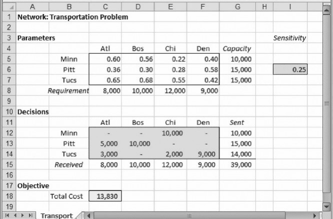
As an illustration, we revisit the transportation problem introduced in Chapter 3.
In Example 3.1 (Goodwin Manufacturing Company), the model allowed us to find the
cost-minimizing distribution schedule in a setting with three plants shipping to four
warehouses. We encountered the optimal solution in Figure 3.2, which is reproduced
in Figure 4.1. The tight supply constraints are the Minneapolis and Pittsburgh
capacities and the optimal total cost in the base case is $13,830.
Suppose that we are using the transportation model as a planning tool and we want
to explore a change in the unit cost of shipping from Pittsburgh to Atlanta, which is
$0.36 in the base case. We might be negotiating with a trucking company over the
charge for shipping, so we want to study a range of alternative values for the PA
cost. Suppose that, as a first step, we are willing to examine a large range of values,
from $0.25 to $0.75. For this purpose we create a cell and enter the formula
=PsiOptParam(0.25,0.75). In Figure 4.1, we have reserved column I for sensi-
tivity parameters, and we enter the formula in cell I6. Then, in C6 we reference cell I6.
The PsiOptParam function displays the minimum value of its range, so the value $0.25
appears in both cell I6 and cell C6. (To restore the model, we would simply enter the
original unit cost of $0.36 in cell C6.)
120
Chapter 4 Sensitivity Analysis in Linear Programs
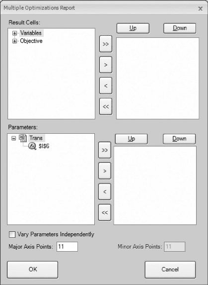
Next, we go to the drop-down menu on the Reports icon in the RSP ribbon and
select Optimization
Q Parameter Analysis. The Multiple Optimizations Report,
shown in Figure 4.2, appears on the screen. In the Multiple Optimizations Report
window, we select the results to track in the upper part of the report and the par-
ameter(s) to vary in the lower part. In particular, we fill out the form by choosing
C18 as the objective function cell and C13:F13 as the variables to track. (These
four cells represent the optimal shipments from the Pittsburgh plant.) Those selections
appear in the upper right-hand window, as shown in Figure 4.3. As a general rule, we
prefer to have the objective function listed first, as shown in the figure. In the bottom
pair of windows, we select cell I6 as the parameter, so that the form looks like the
version shown in Figure 4.3.
Next, we have to specify the number of values between the parameter’s lower
limit of $0.25 and the upper limit of $0.75. If we specify 11 Major Axis Points, as
in Figure 4.3, the step size will be $0.05. (That is, starting at 0.25 and taking steps
of 0.05, the eleventh step will be 0.75.) Finally, we click OK on the form. The program
inserts a new worksheet in our workbook, labeled Analysis Report, and records the
results. Figure 4.4 displays the Parameter Analysis Report, slightly edited for better
readability.
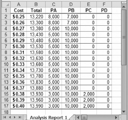
The report shows how the optimal total cost changes and how the optimal
Pittsburgh shipments change as the unit cost of the PA route increases. The first
column of the table gives the values of the unit cost under study, from $0.25 to
$0.75. The second column gives the corresponding optimal total cost. The four
columns C–F, which were selected in Figure 4.3, show the various shipments from
Figure 4.1. Solution for Example 3.1.
4.1. Parameter Analysis in the Transportation Example 121
the Pittsburgh plant. Thus, for the range of unit costs ($0.25–$0.75), four distinct
profiles appear. For values of $0.30 and $0.35, the base case solution prevails
(5000 units to Atlanta and 10,000 units to Boston), but above and below those
values the optimal shipping schedule changes.
†
At a unit cost of $0.25, the PA shipment is 8000 units, and 7000 units are
shipped on the PB route.
†
At unit costs of $0.30 and $0.35, the PA shipment is 5000 units, while 10,000
units are shipped on the PB route. In effect, there is a shift away from the PA
route as its cost rises.
†
At unit costs of $0.40–$0.65, the PA shipment is 3000 units, while 2000 units
are shipped on PC, as well as 10,000 units on PB. Thus, there is a shift away
from the PA route toward an entirely new route.
†
At unit costs of $0.70 and above, the PA route is not used at all.
From this information, we can conclude that the optimal shipping schedule is
insensitive to changes in the PA unit cost, at least between $0.30 and $0.36. Below
that interval, the unit cost could become sufficiently attractive that we would want
Figure 4.2. Initial Multiple Optimizations Report.
122 Chapter 4 Sensitivity Analysis in Linear Programs
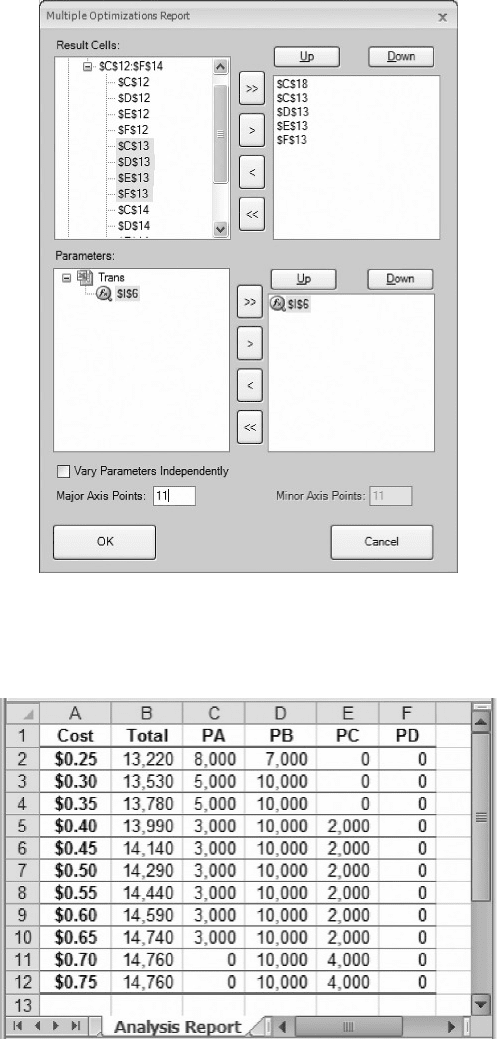
Figure 4.3. Selections in the Multiple Optimizations Report.
Figure 4.4. Parameter Analysis Report for PA unit cost.
4.1. Parameter Analysis in the Transportation Example 123
to shift some shipments to the PA route from PB. Above that interval, however, the unit
cost would become less attractive, and we would eventually want to shift some ship-
ments to the PC route. Subsequently, when the profit contribution reaches approxi-
mately $0.70, we would prefer not to use the PA route at all. Thus, as we face the
prospect of negotiating a unit cost for the PA route, we can anticipate the impact on
Pittsburgh shipments, and on the optimal total cost, from the information in the table.
Because we chose a grid of size $0.05, we don’t know the precise cost interval
over which the optimal shipping schedule remains unchanged. Since the original
unit cost was $0.36, we know that the cost will have to drop to below $0.30 in
order to induce a change in the size of the PA shipment. We also know that a cost
of $0.25 will be sufficient inducement to make a change. The precise cost at which
the change occurs must be somewhere between these two values. We can re-run the
Parameter Analysis Report with a grid of $0.01 to get a better idea of exactly where
the change occurs. One way to do so is to specify new lower and upper limits (such
as 0.25 and 0.40) in the PsiOptParam function and change the number of Major
Axis Points to 16. Figure 4.5 shows the resulting Parameter Analysis Report.
The refined grid shows that the optimal shipments do not change until the unit cost
drops below $0.27 or rises above $0.37. If we wanted to see an even finer grid, we
could produce another report with an even smaller step size. However, we can find
the precise range of “insensitivity” more directly by other means, as we shall see later.
Two important qualitative patterns are visible in Figure 4.4. First, when an objec-
tive function coefficient becomes more attractive, the amount of the corresponding
variable in the optimal solution will either increase or stay the same; it cannot drop.
(However, the increase need not be gradual: The PA shipment jumps from 0 to
Figure 4.5. Parameter Analysis Report on a refined grid.
124 Chapter 4 Sensitivity Analysis in Linear Programs
3000 to 5000 and to 8000 as we read up the table.) Second, when an objective function
coefficient becomes more attractive, the optimal value of the objective function either
stays the same or improves. In this example, the total cost remains unchanged when the
unit cost of the PA route is $0.70 or more; but for $0.65 and below, the total cost
decreases as the PA cost decreases.
In linear programs, a distinct pattern usually appears in sensitivity tables when we
vary a coefficient in the objective function. The optimal values of the decision vari-
ables remain constant over some interval of increase or decrease. Beyond this interval,
a slightly different set of decision variables becomes positive, and some of the
decision variables change abruptly, not gradually. Figure 4.5 illustrates these features
even in the limited portion of the optimal schedule that it tracks.
Solver also offers a Parameter Analysis Report for changes in a RHS constant.
Suppose that, starting from the base case, we wish to explore a change in the
Pittsburgh capacity. (The original figure was 15,000, and at that level, the capacity rep-
resents a scarce resource.) To prepare for this analysis, we first have to determine the
range of values to study, such as 14,000–24,000. Then we devote a cell in the sensi-
tivity area of the spreadsheet, such as I7, to this parameter. In this cell, we enter the
formula
=PsiOptParam(14000,24000), and we reference this cell in G13. (To
make sure that the analysis varies only this capacity, we set cell C6 back to its original
value of $0.36.)
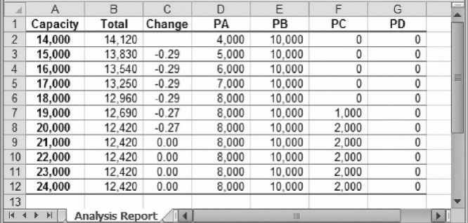
Next, we return to the Reports drop-down menu and ask for an Optimization
Parameter Analysis. Using 11 Major Axis Points, we can examine the effect of increas-
ing Pittsburgh capacity from 14,000 to 24,000 in steps of 1000. The report, slightly
edited, appears in Figure 4.6. The editing consists of making the titles and format
more helpful, but we have manually added column C. The entries in each row of
this column represent the incremental change in the optimal objective divided by
the change in the RHS constant, from the row above. The formula in cell C3 is
=(B2-B3)/(A2-A3), and it has been copied down the column.
Figure 4.6. Parameter Analysis Report for Pittsburgh capacity.
4.1. Parameter Analysis in the Transportation Example 125