Baker R.C. Flow Measurement Handbook: Industrial Designs, Operating Principles, Performance, and Applications

Подождите немного. Документ загружается.

1.A.1 INTRODUCTION 15

1.8 MATHEMATICAL POSTSCRIPT

I have left this note to the end so that those who are not concerned with advanced

mathematical concepts can ignore it.

I have included essential mathematics in the main text of the book. In certain

flowmeters, the mathematical theory is more complex (e.g., the turbine meter),

and the theory has, accordingly, been consigned to an appendix after the relevant

chapter.

One important and interesting mathematical approach, which starts to develop

a unified theory of flow measurement, was first suggested by Shercliff (1962) and

significantly extended by Bevir (1970). Both applied it to electromagnetic flow-

meters where it has been highly successful. Hemp (1975) has also applied this theory

to electromagnetic flowmeters, but he has developed the theory for other types of

flowmeter: ultrasonic (1982), thermal mass (1994a), and Coriolis (1994b, and Hemp

and Hendry 1995). In Chapter 12, on electromagnetic flowmeters, an appendix de-

scribes the essential mathematics. The weight function developed in this theory

provides a measure of the importance of flow in each part of the meter with respect

to the overall meter signal. The flow at each point of a cross-section is weighted with

this function. Ideally the weighting should result in a true summation of the flow

in the meter to obtain a volume flow rate. It has been possible to approach this ideal

for the electromagnetic flowmeter.

For the other types of meters, the reader will be given only a brief explanation

and will be referred to relevant papers. This is partly for want of space in this book

and partly because the theory, although interesting, is still being developed and may

not yet have reached a sufficiently significant stage for the designer.

second mathematical physics theory, first (to my knowledge) applied by Hemp

(1988) to flow measurement, is reciprocity. This, essentially, states that if you apply

a voltage to one end of an electrical network and measure the current at the other

end, you find that by reversing the ends and hence the direction you obtain the

same relationship. Hemp has proposed this as a means of eliminating some errors

in flowmeters to which the theory is applicable.

APPENDIX

1.A

Statistics of Flow Measurement

1.A.1 INTRODUCTION

The main needs of the engineer are to

• understand and be able to give a value to the uncertainty of

particular measure-

ment;

• know how to design a test to provide data of a known uncertainty;

• be able to combine measurements, each with its own uncertainty, into an overall

value; and

INTRODUCTION

• determine the absolute accuracy of an instrument at the end of

traceable ladder

of measurement.

The international and national documents set the recommended approach for

flow metering. Most standard statistics books will provide the essentials (Rice 1988;

cf. Campion et al. 1973, which is often quoted but may not be easy to obtain), but

good school texts may be more accessible (Crawshaw and Chambers 1984, Eccles

et al. 1993a, 1993b). Hayward (1977) is an extremely well written and elegant little

book, which deserves to be updated and reprinted; Kinghorn (1982) provides a well-

written and useful brief review of the main points; and Mattingly (1982) addresses

some of the problems concerned with transfer standards.

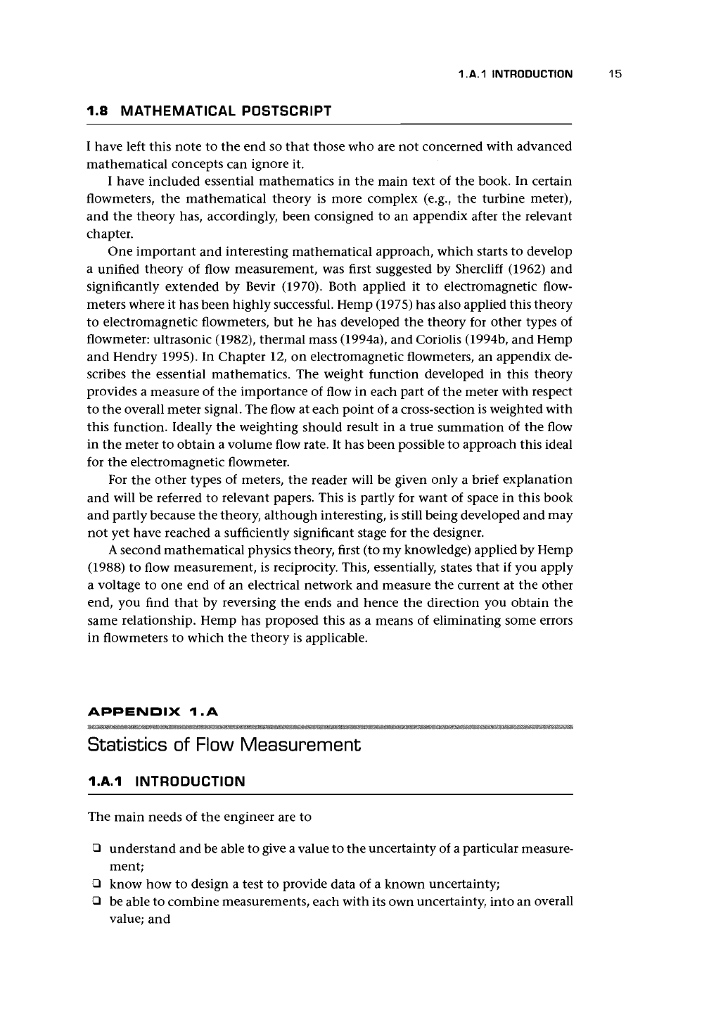
1.A.2 THE NORMAL DISTRIBUTION

The Normal distribution, Figure l.A.l(a), is also known as the Gaussian distribution

after Carl Friedrich Gauss, who proposed it as a model for measurement errors (Rice

1988).

The notation used for the Normal curve is N(/x, a

) which is the distribution

under the curve

<t>(0.5) = 0.6915

PROBABILITY OF READING

LYING IN UNSHADED

AREA = 0.3085

SHADED AREA

- 0.950

ARE A

=0.025

AREA - 0.025

Figure l.A.l. The Normal distribution.

f(*) =

(l.A.l)

where

is the mean value of the data, and

is the variance. Alternatively, a is the

standard deviation for the whole popula-

tion. We can simplify the curve (normalize

it) by putting z = (x

—

fi)/a and obtaining

[Figure l.A.l(b)]

0(z) =

(1.A.2)

With the form of Equation (1.A.2), the

curve does not vary with the size of the pa-

rameters fi and o.

What the curve tells us (in relation to in-

strument measurements) is that the statisti-

cal chance of an instrument reading giving

a value near to the mean /x is high, but the

farther away the reading is from the mean,

the less the chance is of its occurring (indi-

cated by the curve decreasing in height the

further one moves from the mean), and as

values of the reading get farther still from

li, so the chance gets less and less.

The area under the curve of Equation

(1.A.2) [Figure l.A.l(b)], which reaches to

infinity each way, is unity, and this is the

1 .A.3 THE STUDENT t DISTRIBUTION 17

probability of the reading lying within this

curve (obviously). The area under the curve

between z =

—oo

and some other value of z

is given by

—

y/2jT

J-o

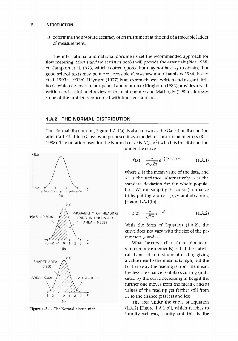
Table l.A.l. A selection of values from

the normal distribution function <f>(z)

Symmetrical Central

z 3Hz) Area Under Curve

(1.A.3)

and is the probability that a reading will lie

within that range and is obtained numeri-

cally and given in Table l.A.l in normalized

form. For instance, if

= 0.5,

<I>(z)

= 0.6915,

where

<I>(z)

is the area under the curve from

z = -oo to z = 0.5 in this case. So the

chance of a reading lying beyond this point

is 0.3085, or about 30%.

We shall be interested in the chance that

a flowmeter reading will fall between cer-

tain limits each side of z = 0, the mean

value.

chance of 95% is often used and is

called a 95% confidence level. This means

that 19 times out of 20 the reading will fall

between the limits. This requires that the

central area of the curve [Figure l.A.l(c)]

has a value of 0.95, or 0.475 each side of

the mean. To obtain z from this value, we need to add 0.475 + 0.5 = 0.975, and this

gives a value (Table l.A.l) of z = 1.96. If we put this in terms of x, we obtain

0.5

1.28

1.282

1.29

1.64

1.645

1.65

1.96

2.57

2.576

2.58

3.29

3.30

0.5000

0.6915

0.8997

0.9000

0.9015

0.9495

0.9500

0.9505

0.9750

0.99492

0.99500

0.99506

0.99950

0.99952

0.80

0.90

0.95

0.99

0.999

After

Lindley and

F. Scott, New Cam-

bridge Statistical

Tables,

2nd ed., Cambridge:

Cambridge Univ. Press. Table 4, pp. 34, 35.

x-ti = 1.96a

(1.A.4)

or the band around the mean value of the reading within which

95%

of the readings

statistically should fall, is approximately ±2a, or two standard deviations from the

mean.

If we are interested, not in the spread of individual readings, but in the spread

of the mean of small sets of readings, a statistical theorem called the Central Limit

Theorem provides the answer. If a sample of n readings has a mean value of M, then

the distribution of means like M

given by N(^, a

/n). This is intuitively reasonable

because one would expect that the scatter of means of groups of n readings would

have a smaller variance, o

In, than the readings themselves, as well as a smaller

standard deviation,

cr/y/n.

In this discussion, we have skated over the need to know

the value of the standard deviation of the whole normal population. If we do not

know o, then we can approximate it with the value of the standard deviation s of

the small set of

So if n > 30, it is usually sufficiently precise to take a

—

s. If n < 30,

the standard deviation should be taken as a = s^Jnj^Jn

—

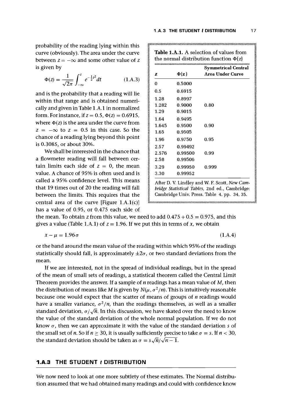
1.A.3 THE STUDENT t DISTRIBUTION

We now need to look at one more subtlety of these estimates. The Normal distribu-

tion assumed that we had obtained many readings and could with confidence know

INTRODUCTION

-4 -3 -2 -1

1.96

2.23

Figure l.A.2. Student's t distribution curves com-

pared with the Normal curve. Note p = 5% as related

to Table l.A.2 for both tails.

that they formed a Normal distribution. We

can agree that if the error is random, then

it is a fair assumption that many readings

would form a Normal distribution. How-

ever, often we have only a few readings,

and these may not be uniformly distributed

within the curve of Figure l.A.l. Too many

may lie outside the 1.96 a limit. For this

reason, we use the Student t distribution,

which allows for small samples on the as-

sumption that the distribution, as a whole,

is Normal. Figure l.A.2 shows the effect of

the small number of readings. Since, with

a small number of readings, one has to be

subtracted from all the others to obtain a

mean, the number of independent values is one less than the number of readings,

and so the statisticians say that there is one less degree of freedom than the number

of readings. In Figure l.A.2, v is the symbol for the degree of freedom, and v =

- 1,

where n is the number of readings. For v -* oo, the t distribution tends to a Normal

curve with mean zero and variance unity.

Figure l.A.2 shows clearly the larger area spreading beyond the Normal curve in

which the readings may lie and the reason for the greater uncertainty. The curves are

used in a similar way to the Normal curve, but, as an alternative, Table l.A.2 provides

the information we need. If we have 10 readings, say, and so select the value of

= 9

for the degree of freedom, and if we wish to find the limits for a confidence level

of 95%, we shall need to use the 5% column. We obtain t = 2.262, which we can

apply to obtain the limits for a 95% confidence of ±2.262 a/y/n on the mean values

of groups of readings, where n is the number of readings in the group. We should

Table l.A.2. A selection of values from the student t function

p(%) (Total)

121

120

3.078

1.886

1.533

1.383

1.328

1.311

1.296

1.289

1.282

p/2

6.314

2.920

2.132

1.833

1.729

1.699

1.671

1.658

1.645

(%) (per tail)

2.5

12.71

4.303

2.776

2.262

2.093

2.045

2.000

1.980

1.960

0.5

63.66

9.925

4.604

3.250

2.861

2.756

2.660

2.617

2.576

0.1

0.05

636.6

31.60

8.610

4.781

3.883

3.659

3.460

3.373

3.291

After

Lindley and

F. Scott, New

Cambridge Statistical

Tables,

2nd

ed., Cambridge: Cambridge Univ. Press, Table 10, p. 45.

1.A.4 PRACTICAL APPLICATION OF CONFIDENCE LEVEL 19

note,

however, that the 95% confidence level from Table 1.A.2 gives a t value that

varies little from 2.0 if v > 20. The limits for 95% confidence will then be ±2.0

on the mean values of groups of readings.

I have always been puzzled by the name Student, but Eccles et

al.

(1993b) explain

that the originator of this technique was William S. Gosset, born 1876, who used

the pseudonym Student.

1.A.4 PRACTICAL APPLICATION OF CONFIDENCE LEVEL

The method described in Section 1.4 leads to the following steps (cf. Hayward 1977):

i. Write down systematic uncertainties and derive the standard uncertainty for

each component,

ii.

Write down random uncertainties and derive the standard uncertainty for each

component,

iii.

Calculate the combined standard uncertainty for uncorrelated input quantities

(and refer to NAM AS 1997 if correlated),

iv. Obtain the expanded uncertainty using k = 2 for 95% confidence.

Taking a simple example, where we need to revert to t, suppose that we obtain

a series of volumetric flow readings from a

mm ID flowmeter with the flow set at

10m

/h:

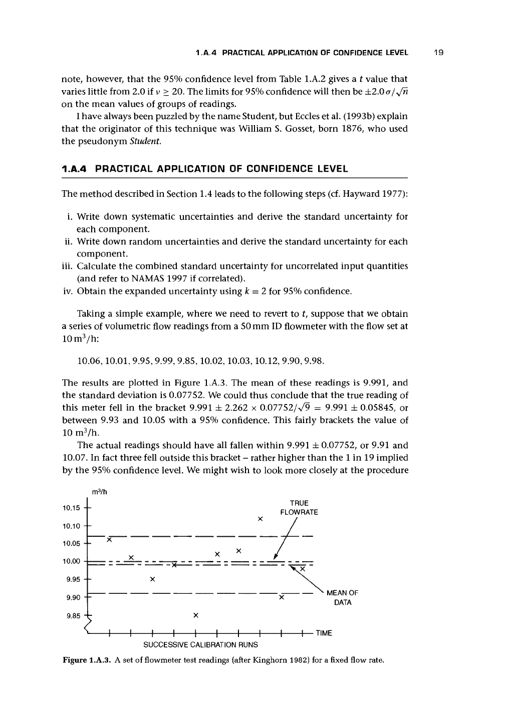
10.06,

10.01,

9.95, 9.99, 9.85, 10.02,10.03,10.12, 9.90, 9.98.

The results are plotted in Figure

l.A.3.

The mean of these readings is

9.991,

and

the standard deviation is 0.07752. We could thus conclude that the true reading of

this meter fell in the bracket 9.991 ± 2.262 x 0.07752/V9 = 9.991 ± 0.05845, or

between 9.93 and 10.05 with a 95% confidence. This fairly brackets the value of

10 m

/h.

The actual readings should have all fallen within 9.991 ± 0.07752, or 9.91 and

10.07.

In fact three fell outside this bracket - rather higher than the 1 in 19 implied

by the 95% confidence level. We might wish to look more closely at the procedure

10.15 --

10.10 --

10.05 +

10.00

9.95 - - X

9.90 -

9.85 + X

' 1 1 1 1 1 1 1 1 1

|—TIME

SUCCESSIVE CALIBRATION RUNS

Figure l.A.3. A set of flowmeter test readings (after Kinghorn 1982) for a fixed flow rate.

INTRODUCTION

for obtaining these results since this suggests a possible problem with the means for

obtaining the data.

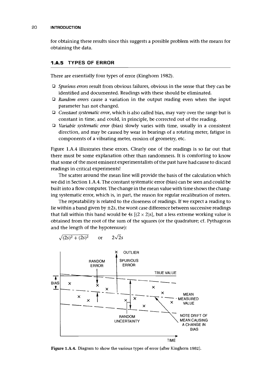
1.A.5 TYPES OF ERROR

There are essentially four types of error (Kinghorn 1982).

•

Spurious errors

result from obvious failures, obvious in the sense that they can be

identified and documented. Readings with these should be eliminated.

• Random

errors

cause a variation in the output reading even when the input

parameter has not changed.

• Constant

systematic

error,

which is also called bias, may vary over the range but is

constant in time, and could, in principle, be corrected out of the reading.

•

Variable

systematic

error

(bias) slowly varies with time, usually in a consistent

direction, and may be caused by wear in bearings of a rotating meter, fatigue in

components of a vibrating meter, erosion of geometry, etc.

Figure 1.A.4 illustrates these errors. Clearly one of the readings is so far out that

there must be some explanation other than randomness. It is comforting to know

that some of the most eminent experimentalists of the past have had cause to discard

readings in critical experiments!

The scatter around the mean line will provide the basis of the calculation which

we did in Section l.A.4. The constant systematic error (bias) can be seen and could be

built into a flow computer. The change in the mean value with time shows the chang-

ing systematic error, which is, in part, the reason for regular recalibration of meters.

The repeatability is related to the closeness of readings. If we expect a reading to

lie within a band given by ±2s, the worst case difference between successive readings

that fall within this band would be 45 [(2 x 2)5], but a less extreme working value is

obtained from the root of the sum of the squares (or the quadrature; cf. Pythagoras

and the length of the hypotenuse):

J{2s)

+ (25)

or 2V25

BIAS

RANDOM

ERROR

OUTLIER

SPURIOUS

ERROR

TRUE VALUE

RANDOM

UNCERTAINTY

MEAN

- MEASURED

VALUE

NOTE DRIFT OF

MEAN CAUSING

A CHANGE IN

BIAS

TIME

Figure l.A.4. Diagram to show the various types of error (after Kinghorn 1982).

1.A.7 UNCERTAINTY RANGE BARS, TRANSFER STANDARDS, AND YOUDEN ANALYSIS

1.A.6 COMBINATION OF UNCERTAINTIES

If we combine uncertainties due to the nature of a flowmeter

;

s operating equation,

then we take the following approach. Suppose that the flowmeter has the equation

n v v

v v

m /-i A r\

Lit) — ^\ ^0 ^3 A

1«A« J I

To obtain the uncertainty in q

, we need the partial derivative of

with respect to X\,

etc. The required result can be achieved, either by differentiating the equation

as it stands or by first taking logarithms of both sides. We shall skip this and go

straight to the result:

)

nu(x

)

u(x

)

mu(x

)

(1.A.6)

The problem with this equation is that the arithmetic sum of the uncertainties is

usually overpessimistic. It is, therefore, recommended that they be combined in

quadrature, or by the root-sum-square (rss) method. This leads to the following

equation:

(nu{x

{

)

\ x

There are complications beyond this

equation. x

may appear in the equation as

*6-

In this case,

will need to be

dealt with first and will require careful con-

sideration as to whether the actual errors in

these quantities are combining, canceling,

or random.

|V^V

FLOW RATE

(a)

(1.A.7)

TRUE

' VALUE

TIME

1.A.7 UNCERTAINTY RANGE

BARS,

TRANSFER STANDARDS,

AND YOUDEN ANALYSIS

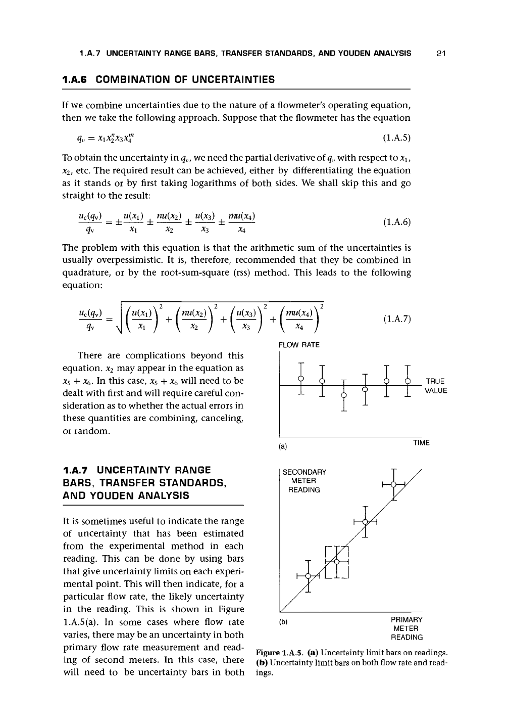
It is sometimes useful to indicate the range

of uncertainty that has been estimated

from the experimental method in each

reading. This can be done by using bars

that give uncertainty limits on each experi-

mental point. This will then indicate, for a

particular flow rate, the likely uncertainty

in the reading. This is shown in Figure

l.A.5(a). In some cases where flow rate

varies, there may be an uncertainty in both

primary flow rate measurement and read-

ing of second meters. In this case, there

will need to be uncertainty bars in both

SECONDARY

METER

READING

(b)

PRIMARY

METER

READING

Figure l.A.5. (a) Uncertainty limit bars on readings.

(b) Uncertainty limit bars on both flow rate and read-

ings.

INTRODUCTION

71.7r

71.6

= 71.5445

71.5

71.4

MAY MAY JUN SEP NOV DEC JAN FEB FEB

| 3 | 20 | 7 | 28 | 17 | 21 | 6 | 8 I 4 |

DATE

(a)

1.005

1.004

1.00372

1.003

(b)

(C)

1.002

2cr

MAY MAY JUN SEP NOV DEC JAN FEB FEB

1-3 1 20 1 7 1 28 | 17 I 21 | 6 I 2 I 4 I

DATE

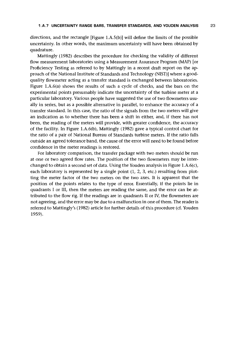
Figure l.A.6. Turbine meter as a transfer standard (from Mattingly 1982; repro-

duced with the author's permission), (a) Typical turbine meter control chart

for meter factor, (b) Typical turbine meter control chart for ratio, (c) Graphical

representation of the Youden plot.

1.A.7 UNCERTAINTY RANGE BARS, TRANSFER STANDARDS, AND YOUDEN ANALYSIS 23

directions, and the rectangle [Figure l.A.5(b)] will define the limits of the possible

uncertainty. In other words, the maximum uncertainty will have been obtained by

quadrature.

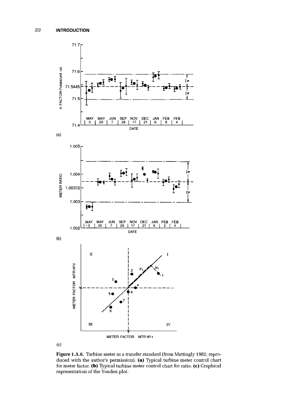
Mattingly (1982) describes the procedure for checking the validity of different

flow measurement laboratories using a Measurement Assurance Program (MAP) [or

Proficiency Testing as referred to by Mattingly in a recent draft report on the ap-

proach of the National Institute of Standards and Technology (NIST)] where a good-

quality flowmeter acting as a transfer standard is exchanged between laboratories.

Figure l.A.6(a) shows the results of such a cycle of checks, and the bars on the

experimental points presumably indicate the uncertainty of the turbine meter at a

particular laboratory. Various people have suggested the use of two flowmeters usu-

ally in series, but as a possible alternative in parallel, to enhance the accuracy of a

transfer standard. In this case, the ratio of the signals from the two meters will give

an indication as to whether there has been a shift in either, and, if there has not

been, the reading of the meters will provide, with greater confidence, the accuracy

of the facility. In Figure l.A.6(b), Mattingly (1982) gave a typical control chart for

the ratio of a pair of National Bureau of Standards turbine meters. If the ratio falls

outside an agreed tolerance band, the cause of the error will need to be found before

confidence in the meter readings is restored.

For laboratory comparison, the transfer package with two meters should be run

at one or two agreed flow rates. The position of the two flowmeters may be inter-

changed to obtain a second set of data. Using the Youden analysis in Figure l.A.6(c),

each laboratory is represented by a single point (1, 2, 3, etc.) resulting from plot-

ting the meter factor of the two meters on the two axes. It is apparent that the

position of the points relates to the type of error. Essentially, if the points lie in

quadrants I or III, then the meters are reading the same, and the error can be at-

tributed to the flow rig. If the readings are in quadrants II or IV, the flowmeters are

not agreeing, and the error may be due to a malfunction in one of them. The reader is

referred to Mattingly's (1982) article for further details of this procedure (cf. Youden

1959).

CHAPTER

Fluid Mechanics Essentials

2.1 INTRODUCTION

In a recent book (Baker 1996), I provided an introduction to fluid mechanics and

thermodynamics, particularly aimed at instrumentation.

do not, therefore, propose

to repeat what is written there but rather to confine myself to essentials. In addition,

Noltingk (1988) has provided

very valuable handbook on general instrumentation.

In this book, I shall use the term fluid to mean liquid or gas and will refer to either

liquid or gas only when the more general term does not apply.

2.2 ESSENTIAL PROPERTY VALUES

Flowmeters generally operate in a range of fluid temperature from — 200°C (-330°F)

to 500°C (930°F), with line pressures up to flange rating for certain designs. Typical

values of density and viscosity are given in Table 2.1.

It should also be noted that liquid viscosity decreases with temperature, whereas

gas viscosity increases with temperature at moderate pressures. In common fluids,

such as air and water, the value of viscosity

not dependent on the shear taking place

in the flow. These fluids are referred to as Newtonian in their behavior as compared

with others where the viscosity is a function of the shear taking place. The behavior

of such fluids, known as non-Newtonian, is very different from normal fluids like

water and air. Newtonian fluid behavior is a good representation for the behavior of

the bulk of fluids.

2.3 FLOW IN A CIRCULAR CROSS-SECTION PIPE

An essential dimensionless parameter that defines the flow pattern at a particular

value of the parameter is the Reynolds number

where p is the density of the fluid,

\±

is the dynamic viscosity, and, when applied

to flow measurement, V is the velocity in the pipe, and D is the pipe diameter.

Typical values of Reynolds number are: for water with /x/p = 10~

/s, V =1 m/s

(3.3 ft/s), D = 0.1 m (4 in.) Re= 10

; and for air at ambient conditions with /x/p =

1.43 x 10-

/s,

= 10 m/s (33 ft/s), D = 0.1 m (4 in.)

= 0.7 x 10