Baumgarte T., Shapiro S. Numerical Relativity. Solving Einstein’s Equations on the Computer
Подождите немного. Документ загружается.


5.2 Hydrodynamics 151
Exercise 5.24 Prove the relationship between the components of the electromag-
netic fields as measured by a normal observer and by an observer at rest in the
fluid:
E
a
=−
abc
u
b
B
(u)
c
, (5.129)
B
a
=−n
b
u
b
B
a
(u)
+ n
b
B
b
(u)
u
a
. (5.130)
To derive the magnetic field evolution equations, introduce the dual of the Faraday tensor
according to
F
∗ab
=
1
2
abcd
F
cd
. (5.131)
Exercise 5.25 Show that
B
a
(u)
=−F
∗ab
u
b
. (5.132)
Substituting equation (5.126) into equation (5.131) yields
F
∗ab
= u
b
B
a
(u)
− u
a
B
b
(u)
. (5.133)
Inserting equation (5.133) into the “magnetic” Maxwell equations, ∇
a
F
∗ac
= 0, yields
∂
a
(−g)
1/2
u
c
B
a
(u)
− u
a
B
c
(u)
= 0, (5.134)
or
∂
a
γ
1/2
W
(
v
c
b
a
− v
a
b
c
)
= 0, (5.135)
wherewehavedefined
b
a
≡ B
a
(u)
/(4π)
1/2
(5.136)
and v
a
= u
a
/u
t
. We can now split the above equation into two pieces by introducing the
magnetic field variable
B
i
= (4π )
1/2
γ
1/2
W (b
i
− v
i
b
t
). (5.137)
The variable
B
i
is essentially the spatial component of the magnetic field B
i
as measured
by a normal observer, as shown in the next exercise.
Exercise 5.26 Show the relation
B
i
= (γ )
1/2
B
i
. (5.138)
Setting the index c = t in equation (5.135) yields the magnetic constraint equation,
∂
i
B
i
= 0 (5.139)
(i.e., D
i
B
i
= 0), the condition for “no magnetic monopoles”. Setting c = i yields the
magnetic evolution (induction) equation,
∂
t
B
i
− ∂
j
v
i
B
j
− v
j
B
i
= 0. (5.140)
152 Chapter 5 Matter sources
Integrating this set of equations together with the fluid equations typically forces us to
translate between the two sets of magnetic variables, b
a
and B
i
. The components of b
a
are best obtained by solving equation (5.137) together with the orthogonality relation
b
a
u
a
= 0.
Analytically, the magnetic induction equation preserves the constraint condition (5.139)
if the constraint is satisfied on the initial time slice, but considerable care must be taken to
ensure that this happens in a numerical evolution. Defining a vector potential A
i
accord-
ing to B
i
=
ijk
D
j
A
k
and evolving A
i
instead of B
i
automatically guarantees that the
constraint will be satisfied, but the resulting evolution equation for A
i
introduces a second-
order spatial derivative term that can make the numerical evolution too diffusive. High-
order finite difference schemes for evolving the induction equation while maintaining the
divergence constraint to roundoff precision are called constrained transport schemes.
41
One version, called flux-interpolated constrained transport,
42
consists in replacing the
induction equation flux computed at each spatial grid point with linear combinations of
the flux computed at that point and neighboring points. The combination assures both that
second-order accuracy is maintained and that the constraint D
i
B
i
= 0 is strictly enforced.
Another means of maintaining this divergence constraint is called hyperbolic divergence
cleaning
43
and involves adding a new scalar field to the induction equation as well as a new
hyperbolic equation containing D
i
B
i
to describe the evolution of this new field. The role of
the new system is to transport divergence errors to the computational domain boundaries
with maximal allowable speed, while simultaneously damping them.
The electromagnetic field equations derived in the ideal MHD limit above are consid-
erably simpler to treat than the full set of Maxwell’s equations without approximation.
However, there are regimes when it becomes necessary to work with Maxwell’s equations
in full generality. For example, when an electromagnetic field reaches the surface of a star
and then propagates out into the exterior vacuum, the fields are no longer frozen into in
a highly conducting plasma and the MHD approximation breaks down. The general form
of Maxwell’s equations can be cast into 3 +1 form, which facilitates their integration in
conjunction with 3 +1 equations for the gravitational field. Begin by decomposing the
electromagnetic current 4-vector J
a
according to
J
a
= n
a
ρ
e
+ j
a
, (5.141)
where ρ
e
and j
a
are the charge density and spatial current as observed by a normal observer
n
a
( j
a
n
a
= 0). With these definitions, Maxwell’s equations,
∇
b
F
ab
= 4π J
a
, (5.142)
and
∇
[a
F
bc]
= 0, (5.143)
41
Evans and Hawley (1988).
42
T
´
oth (2000).
43
See, e.g., Dedner et al. (2002) and references therein.
5.2 Hydrodynamics 153
can be brought into 3 + 1 form as follows:
44
D
i
E
i
= 4πρ
e
(5.144)
∂
t
E
i
=
ijk
D
j
(α B
k
) − 4παj
i
+ αKE
i
+ L
β
E
i
(5.145)
D
i
B
i
= 0 (5.146)
∂
t
B
i
=−
ijk
D
j
(αE
k
) + α KB
i
+ L
β
B
i
. (5.147)
Exercise 5.27 Verify the 3 + 1 form of Maxwell’s equations given above.
The charge conservation equation,
∇
a
J
a
= 0, (5.148)
which is implied by equation (5.142), becomes
∂
t
ρ
e
=−D
i
(αj
i
) + α Kρ
e
+ L
β
ρ
e
. (5.149)
Exercise 5.28 Show that the familiar form of Maxwell’s equations in special relativ-
ity can be recovered easily by evaluating equations (5.144)–(5.147) for a Minkowski
spacetime with γ
ij
= η
ij
,whereη
ij
is the flat spatial metric in an arbitrary coordinate
system, α = 1, K = 0andβ
i
= 0.
Exercise 5.29 Derive the MHD induction equation (5.140) from equation (5.147).
Hint: Take the trace of the 3 + 1 evolution equation for ∂
t
γ
ij
and combine it with
the Lie derivative
L
β
B
i
to give
αKB
i
+ L
β
B
i
= D
j
(β
j
B
i
− β
i
B
j
) − B
i
∂
t
ln γ
1/2
, (5.150)
where we have used the magnetic constraint (5.146). Substitute (5.150) together with
the ideal MHD equation (5.128) into Faraday’s law (5.147) to get the result.
When treating an electromagnetic field at the boundary between a highly conducting
plasma and a vacuum, such as at the surface of a star, the required electromagnetic field
evolution equations switch from being the MHD induction equation for the magnetic field
in the matter interior to the full set of B-field and E-field evolution equations in the vacuum
exterior. Boundary conditions for B
i
and E
i
just outside the surface are necessary to extend
the integrations into the exterior. These boundary values may be obtained by matching
fields across the surface using the familiar “junction conditions” of electrodynamics in the
rest-frame of the fluid at the surface.
45
It is computationally simpler, and in some cases it may even be more appropriate, to
treat the region outside the surface of a star as an extended atmosphere of very low-density
plasma, in which case the MHD approximation may still hold. In the end, the choice
depends on the physical situation, as well as the specific questions, being addressed.
44
See, e.g., Thorne and MacDonald (1982).
45
See, e.g., Misner et al. (1973), Section 21.13.

154 Chapter 5 Matter sources
Equations of baryon, energy and momentum conservation
The evolution equations for an MHD plasma are straightforward generalizations of the
hydrodynamical equations derived earlier in this chapter for a nonmagnetic gas. In the
MHD limit the electromagnetic piece of the total energy-momentum tensor can be written
in terms of b
a
according to
T
ab
em
= b
2
u
a
u
b
+
1
2
b
2
g
ab
− b
a
b
b
, (5.151)
where b
2
= b
a
b
a
.
Exercise 5.30 Show that in the MHD limit, the electromagnetic source terms
appearing in the 3 + 1 gravitational field equations can be expressed in terms of b
a
as follows:
ρ
em
= b
2
W
2
−
1
2
− (αb
t
)
2
, (5.152)
S
em
i
= b
2
u
i
W − αb
t
b
i
, (5.153)
S
em
ij
= b
2
u
i
u
j
+
1
2
γ
ij
− b
i
b
j
, (5.154)
S
em
= b
2
γ
ij
u
i
u
j
+
3
2
− γ
ij
b
i
b
j
. (5.155)
Equation (5.12) expressing baryon conservation and equation (5.13) expressing energy
conservation for a perfect gas (or equation 5.19 for a -law EOS) remain unchanged.
The reason that the energy equation is unchanged is that there is no Joule heating by the
electromagnetic field in the MHD limit (see exercise 5.31 below).
Exercise 5.31 (a) Use equations (5.116), (5.142)and(5.143) to show that the
equations of motion of the electromagnetic field satisfy
∇
a
T
ab
em
=−F
bc
J
c
. (5.156)
(b) Use this relation to show that, in the presence of an electromagnetic field,
equation (5.13) becomes
∂
t
(γ
1/2
E) + ∂
j
(γ
1/2
Ev
j
) =
− P
∂
t
(γ
1/2
W ) +∂
i
(γ
1/2
W v
i
)
−
αγ
1/2
u
b
F
bc
J
c
, (5.157)
while equation (5.19) becomes
∂
t
(γ
1/2
E
∗
) + ∂
j
(γ
1/2
E
∗
v
j
) =−u
b
F
bc
J
c
E
∗
W
(1−)
αγ
1/2
. (5.158)
(c) Argue that, in the case of a perfect conductor, the terms involving J
a
in the above
equations vanish.

5.2 Hydrodynamics 155
The equation of momentum conservation may be written in terms of the 4-vector S
∗
a
,a
generalization of the momentum-density S
a
defined in equation (5.10) in the absence of a
magnetic field:
S
∗
a
= (ρ
0
h + b
2
)Wu
a
. (5.159)
Exercise 5.32 Show that S
i
, the momentum density appearing as a source term in
the 3 + 1 gravitational field equations and defined in equation (5.1), is given by
S
i
= (ρ
0
h + b
2
)Wu
i
− αb
i
b
t
, (5.160)
and is thus not equal to S
∗
i
in general.
The equation of momentum conservation, obtained from ∇
a
T
a
b
= 0, is then a general-
ization of equation (5.14) and may be written in the form
46
∂
t
γ
1/2
S
∗
i
− αb
i
b
t
+ ∂
j
γ
1/2
S
∗
i
v
j
− αb
i
b
j
=
− αγ
1/2
∂
i
P +
b
2
2
+
1
2
S
∗
a
S
∗
c
αS
∗t
− αb
a
b
c
∂
i
g
ac
. (5.161)
There are alternative ways to cast the basic MHD equations, all of which are equivalent
analytically but are quite different when implemented numerically. For example, another
way of writing the momentum conservation equation is to use equation (5.156)intheform
∇
b
T
ab
fluid
=−∇
b
T
ab
em
= F
ab
J
b
to get
47
∂
t
(γ
1/2
S
fluid
i
) + ∂
j
(γ
1/2
S
fluid
i
v
j
) =
− αγ
1/2
∂
i
P +
S
fluid
a
S
fluid
b
2αS
t
fluid
∂
i
g
ab
+ αγ
1/2
F
ia
J
a
, (5.162)
where S
fluid
a
isgivenbyequation(5.10). The above expression exhibits the relativistic
generalization of the familiar J × B Newtonian force term on the right-hand side.
Exercise 5.33 Show that the electromagnetic term appearing on the right-hand side
of equation (5.162) may be expanded in terms of the normal field components E
i
and B
i
to give
αγ
1/2
F
ia
J
a
= α
γ
1/2
4π
E
i
(D
j
E
j
) (5.163)
−
γ
1/2
4π
B
j
jik
(∂
t
E
k
− β
l
∂
l
E
k
+ E
l
∂
l
β
k
− αKE
k
) + ∂
i
(α B
j
) − ∂
j
(α B
i
)
.
Note that there is a nasty time derivative of the electric field appearing on the right-hand
side of equation (5.163). This is probably the most challenging term in equation (5.162)for
numerical implementation, although it is
O(v
2
/c
2
) times smaller than the last two terms
46
De Villiers and Hawley (2003).
47
Wilson (1975); Sloan and Smarr (1985); Baumgarte and Shapiro (2003b).
156 Chapter 5 Matter sources
on the right-hand side of equation (5.163) and is likely to be small in most applications.
In such cases, it may be useful to invoke “operator splitting” to estimate this term by
extrapolating from the two previous timesteps, integrate the resulting system of equations,
use the result to improve the estimate of this term, and then iterate. Such an approach, or
some other low-order approximation, may be adequate to account for the contribution of
this term. Alternatively, it simply might be preferable to use equation (5.161) in lieu of
equation (5.162) to avoid the extra time derivative term.
Exercise 5.34 Here you will take the Newtonian limit to recover a familiar
expression for the Newtonian MHD equation of momentum conservation. Take
g
00
→−(1 +2), where is the Newtonian potential, to find
1
2
S
fluid
a
S
fluid
b
αS
t
fluid
∂
i
g
ab
→−
1
2
ρ∂
i
g
00
= ρ∂
i
. (5.164)
Then evaluate equation (5.162) in the Newtonian limit to obtain in Cartesian coor-
dinates (γ
1/2
= 1)
∂
t
S
fluid
i
+ ∂
j
(S
fluid
i
v
j
)
=−∂
i
P − ρ∂
i
+ ρ
e
E
i
−
1
8π
∂
i
(B
j
B
j
) +
1
4π
B
j
∂
j
B
i
, (5.165)
where S
i
fluid
→ ρv
i
, or, equivalently,
ρ
dv
i
dt
=−∂
i
(P + P
M
) − ρ∂
i
+
1
4π
B
j
∂
j
B
i
+ ρ
e
E
i
. (5.166)
Here we have introduced the Lagrangian time derivative d/dt = ∂
t
+ v
j
∂
j
,defined
the magnetic pressure
P
M
≡
B
2
8π
, B
2
≡ B
j
B
j
, (5.167)
and used Maxwell’s constraint equation ∇
i
E
i
= 4πρ
e
for the electric field. Note that
for a neutral plasma ρ
e
= 0, so that the electric field E
a
disappears entirely from the
above Newtonian equation.
Neither equation (5.161) nor equation (5.162) is in flux-conservative form. To obtain the
equation in conservative form we must evolve the total stress-energy tensor T
ab
directly
and solve algebraically for the primitive variables.
48
The desired system has the identical
form as equations (5.26)–(5.29) derived earlier, only now the total stress-energy tensor
T
ab
is given by equations (5.118) and (5.151), and
˜
S
j
= γ
1/2
S
i
employs equation (5.160)
for the total momentum density. The goal of the numerical evolution is to integrate the
combined system (5.26) and (5.140) for the conservative fluid and magnetic field variables
U = (
˜
D,
˜
S
j
, ˜τ,
˜
B
i
), where
˜
B
i
≡ γ
1/2
B
i
= B
i
, and then combine these variables at each
48
Koide et al. (1999); Komissarov (1999); Gammie et al. (2003); Duez et al. (2005b); Shibata and Sekiguchi (2005);
Del Zanna et al. (2007).

5.2 Hydrodynamics 157
Box 5.1 The relativistic MHD equations
The coupled set of relativistic MHD equations can be written in conservative form as follows:
∂
t
ρ
∗
+ ∂
j
(ρ
∗
v
j
) = 0, (5.168)
∂
t
˜
S
i
+ ∂
j
(α
√
γ T
j
i
) =
1
2
α
√
γ T
ab
g
ab,i
, (5.169)
∂
t
˜τ + ∂
i
(α
2
√
γ T
0i
− ρ
∗
v
i
) = s
˜τ
, (5.170)
∂
t
˜
B
i
+ ∂
j
(v
j
˜
B
i
− v
i
˜
B
j
) = 0, (5.171)
where
ρ
∗
= γ
1/2
αu
t
ρ
0
= γ
1/2
D, T
ab
= (ρ
0
h + b
2
)u
a
u
b
+ (P + b
2
/2)g
ab
− b
a
b
b
, (5.172)
˜τ isgivenbyequation(5.27), s
˜τ
isgivenbyequation(5.32),
˜
S
i
= γ
1/2
S
i
isgivenbyequation(5.160)
and where
b
a
≡ B
a
(u)
/(4π)
1/2
, b
2
≡ b
a
b
a
. (5.173)
To obtain the comoving magnetic field B
a
(u)
, hence b
a
, from the evolved normal field B
a
,where
˜
B
i
≡ γ
1/2
B
i
= B
i
, introduce the projection operator P
ab
= g
ab
+ u
a
u
b
to write
B
a
(u)
=−
P
a
b
B
b
n
c
u
c
, (5.174)
from which one obtains
B
0
(u)
= u
i
B
i
/α, B
i
(u)
=
B
i
/α + B
0
(u)
u
i
u
t
. (5.175)
For a nonmagnetic gas, the above MHD equations reduce to the equations of relativistic hydrody-
namics in conservative form given by equations (5.26)–(5.29).
time step to solve algebraically for the primitive variables P = (ρ
0
,v
i
, P, B
i
). We collect
the coupled set of MHD evolution equations in conservative form
49
in Box 5.1.
As in the nonmagnetic case, highly accurate shock-capturing methods can be applied
to solve this set of equations. No artificial viscosity is needed, in contrast to the case
for nonconservative schemes. However, recovering P by inverting the system of algebraic
equations
U = U (P) can be computationally expensive. Finally, Einstein’s equations in
3 + 1 form must be integrated simultaneously to determine the spacetime metric.
Tests
Komissarov
50
has proposed a suite of challenging one-dimensional tests for relativistic
MHD codes in Minkowski spacetime. The tests involve the propagation of nonlinear,
49
Duez et al. (2005b).
50
Komissarov (1999).
158 Chapter 5 Matter sources
0
1
2
3
4
5
6
0.5 1 1.5 2
x
0
–
10
–
20
–
30
10
20
30
u
y
u
x
B
z
B
y
Figure 5.2 Nonlinear Alfv
´
en wave test for an MHD fluid obeying a -law EOS with = 4/3. Symbols show
simulation results with resolution x = 0.01 and solid lines give the exact solution. The profiles are shown at
time t = t
final
= 2.0. The computational domain is x ∈ (−2, 2). Only the region 0.3 ≤ x ≤ 2.0 is shown in this
graph. [From Duez et al. 2005b.]
relativistic MHD waves in a gas obeying a -law EOS. Most of the tests start with
discontinuous initial data at x = 0, with homogeneous profiles in either half-space. Some
of the tests involve shocks, others represent rarefaction waves. Exact solutions exist for all
the results
51
and can be used for code calibration.
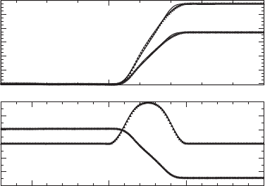
One useful test for a relativistic MHD code in flat spacetime is the propagation of a
nonlinear Alfv
´
en wave, which is a transverse hydromagnetic wave. Such a wave travels
along magnetic field lines similar to the way in which a wave propagates along an elastic
string under tension when it is plucked. The initial data for this test consist of left (x <
−W/2) and right (x > W/2) fluid states separated by a width W = 0.5att = 0. The two
states are joined by continuous functions in the region x ∈ (−W/2, W/2) at t = 0.
52
The
resulting fluid-field pattern propagates with a constant speed in the x-direction. Figure 5.2
shows the results of a simulation using a HRSC scheme that evolves both the fluid and the
radiation field relativistic MHD code.
There are no discontinuities in this problem, so errors should converge to second order
in x for a code that is second-order accurate.
53
To demonstrate this, consider a grid
function g with error δg = g − g
exact
. Calculate the L1 norm of δg (the “average” of δg)
by summing over every grid point i:
L1(δg) ≡ x
N
i=1
|g
i
− g
exact
(x
i
)|, (5.176)
where N ∝ 1/x is the number of grid points. Figure 5.3 shows the L1 norms of the errors
in u
x
, u
y
, B
y
and B
z
at t = t
final
= 2.0. From the figure we conclude that the errors in u
x
,
51
See, e.g., Komissarov (1999); Cabannes (1970).
52
See Komissarov (1997)orDuez et al. (2005b) for details of the setup of initial data together with an analytic solution.
53
See Chapter 6.4 for a discussion of code validation and convergence.
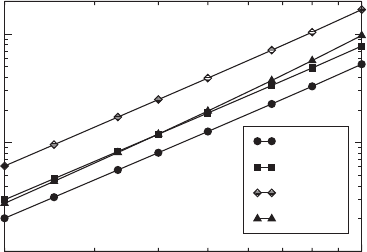
5.2 Hydrodynamics 159
0.01
∆x
0.001
0.01
0.1
L1(δu
x
)
L1(δu
y
)
L1(δB
y
)
L1(δB
z
)
0.002 0.005
Figure 5.3 L1 norms of the errors in u
x
, u
y
, B
y
and B
z
for the nonlinear Alfv
´
en wave test at t = t
final
= 2.0.
This log-log plot shows that the L1 norms of the errors in u
x
, u
y
and B
y
are proportional to (x)
2
, and are thus
second-order convergent. The error in B
z
goes as a slightly higher power of x.[FromDuez et al. 2005b.]
u
y
and B
y
converge at second order in x. The error in B
z
converges at slightly better
than second order in x.
Next, for many applications in numerical relativity it is important to test that a relativistic
MHD code can evolve the equations accurately in the strong gravitational field of a black
hole. One such test checks that the code can maintain stationary, adiabatic, spherical
accretion onto a Schwarzschild black hole, in accord with the relativistic Bondi accretion
solution.
54
In particular, the relativistic Bondi solution is unchanged in the presence of a
divergence-free radial magnetic field. This solution provides a useful diagnostic both for
a numerical scheme that evolves the MHD equations in a fixed background metric as well
as for one that evolves the spacetime metric self-consistently.
55
To test the capability of a code to handle truly dynamical gravitational and MHD
fields simultaneously, one can consider a gravitational wave oscillating in an initially
homogeneous, uniformly magnetized fluid. The gravitational wave will, in general, induce
Alfv
´
en and magnetosonic waves.
56
Duez et al. (2005a) have performed a detailed analysis
of this problem and provide an analytic solution for the perturbations in a form which is
suitable for comparison with numerical results.
This test problem is 1-dimensional. Consider a linear, standing gravitational wave whose
amplitude varies in the z-direction:
h
+
(t, z) = h
+0
sinkz coskt, (5.177)
h
×
(t, z) = h
×0
sinkz coskt, (5.178)
54
Shapiro and Teukolsky (1983), Appendix G.
55
See De Villiers and Hawley (2003)andGammie et al. (2003) for implementations of the Bondi test employing a fixed
background metric, and Duez et al. (2005b) for an implementation in which the metric is evolved.
56
Moortgat and Kuijpers (2003, 2004); K
¨
allberg et al. (2004).
160 Chapter 5 Matter sources
where k is the wave number, and h
+0
and h
×0
are constants. Assume that at t = 0, the
magnetized fluid is unperturbed:
P(0, z) = P
0
,ρ
0
(0, z) = ρ
0
, (5.179)
v
i
(0, z) = 0, B
i
(0, z) = B
i
0
. (5.180)
Subsequently, the gravitational wave excites the MHD modes of the fluid. The gravitational
wave is unaffected by the fluid to linear order, and the metric perturbation, h
µν
(t, z), in the
transverse-traceless (TT) gauge can be calculated from equations (5.177) and (5.178). The
perturbations in pressure δ P(t, z), velocity δv
i
(t, z), and magnetic field δ B
i
(t, z) can be
computed analytically. The solution
57
remains valid as long as we are in the linear regime.
It is a superposition of the three eigenmodes of the homogeneous system (Alfv
´
en, slow
magnetosonic and fast magnetosonic waves), plus a particular solution that oscillates at
the frequency of the gravitational wave.
The numerical simulation
58
adopts geodesic slicing (α = 1,β
i
= 0). The fluid evolves
with a -law EOS with = 4/3. The computational domain is z ∈ (−1, 1) and spans
two wavelengths of the gravitational wave (k = 2π ) and is covered by 200 grid points in
the z-direction. At time t = 0,themetricisgivenbyg
ab
(0, z) = η
ab
+ h
ab
(0, z), where
η
ab
= diag(−1, 1, 1, 1) is the Minkowski metric, and the nonzero components of h
ab
(0, z)
are
h
xx
(0, z) =−h
yy
(0, z) = h
+
(0, z), (5.181)
h
xy
(0, z) = h
yx
(0, z) = h
×
(0, z). (5.182)
Periodic boundary conditions are enforced on both the matter and gravitational field
quantities at the upper and lower boundaries in z.
Figure 5.4 shows a comparison between the analytic solution and numerical simulation
for three selected perturbed variables. The simulation employs the same HRSC relativistic
MHD code used to generate Figures 5.3 and 5.4 and couples it to a general relativistic
3 + 1 BSSN scheme to evolve the metric.
59
Good agreement is shown for the MHD
variables over many periods of the gravitational wave. Good agreement is also found for
the metric perturbations. The pressure perturbation, however, is seen to differ from the
analytic solution by a slight secular drift. (In fact, all variables eventually exhibit a drift
away from the analytic solution, but the drift is first noticeable in the case of the pressure.)
This secular drift is not due to numerical error, but rather is an effect of the nonlinear
terms which are neglected in the analytic solution. To demonstrate that it is not a numerical
error, simulations at resolutions of 50, 100, and 200 grid points were performed, and
convergence was obtained to second order to a solution with nonzero drift. Since the
discrepancy is due to nonlinear terms, choosing smaller initial mass-energy density and
57
Duez et al. (2005a).
58
Duez et al. (2005b).
59
See Chapter 11.5 for a description of the BSSN scheme for the evolution of the gravitational field.