Baumgarte T., Shapiro S. Numerical Relativity. Solving Einstein’s Equations on the Computer

Подождите немного. Документ загружается.

5.4 Scalar ﬁelds 181

ϕ is called an “inﬂaton” scalar ﬁeld. The same equation is also invoked as the evolution

equation for a simple candidate for a dynamical source of dark energy.

A popular interaction potential used in many studies is a quartic self-interaction, which

has the form

int

(ϕ) =

λϕ

, (5.257)

where λ is a dimensionless coupling constant. While this interaction is often employed

for illustrative purposes, plausible models arising in particle physics, like the Higgs ﬁeld

in standard electroweak theory, do contain ϕ

interactions. The only other possibility

for models involving only scalar ﬁelds is an interaction of the form ϕ

, since theories

containing ϕ

are not renormalizable for n > 4.

Much of the astrophysically relevant work on scalar ﬁelds in asymptotically ﬂat space-

times involves complex scalar ﬁelds. Part of the reason is that massive complex ﬁelds can

form stationary equilibrium conﬁgurations (boson stars). The stress-energy tensor for a

massive, self-interacting complex ﬁeld is

(

∇

∇



∗

+∇

∇



∗

)

− g

(

∇

∇



∗

)

− g

V (, 

∗

). (5.258)

The corresponding equations of motion are

∇

 − m

 − λ||

 = 0 (5.259)

and its complex conjugate. Here we have assumed V (, 

∗

) =

|

∗

λ|

∗

The complex scalar ﬁeld can be split into two real scalar ﬁelds according to  = ϕ

+ i ϕ

where ϕ

and ϕ

are real scalar functions. The two real, coupled, second-order equations

that result may then be cast into ﬁrst-order form by introducing new variables as in

equation (5.250) and proceeding in a similar fashion.

As a ﬁnal twist, we can endow the complex scalar ﬁelds with charge e,aswellasmass

m, and allow them to interact with an electromagnetic ﬁeld. Express the Faraday tensor for

the electromagnetic ﬁeld, F

, in terms of the electromagnetic vector potential, A

=∇

−∇

. (5.260)

Deﬁne the operator

≡∇

+ ieA

. The total stress-energy tensor for this system then

becomes

∗



∗

)(D

) +

)(D

∗



∗

) −

)(D

c∗



∗

) − g

V (, 

∗

)

4π

−

16π

(5.261)

See Carroll (2004), Chapter 8.7 and 8.8, for a discussion.

See, e.g., Peskin and Schroeder (1995) for a discussion.

182 Chapter 5 Matter sources

where V (, 

∗

) =

|

∗

|+V

int

(, 

∗

). The corresponding equations of motion

for the scalar ﬁelds are

∇

 + ieA

(2∇

 + ieA

) + ie∇

− 2

∂V (, 

∗

)

∂

∗

= 0, (5.262)

and its complex conjugate, while Maxwell’s equations for the electromagnetic ﬁeld are

∇

= 4π J

, (5.263)

where the conserved 4-current J

is given by

= ie

D

∗

 − 

∗



. (5.264)

Recall that the remaining Maxwell equations, ∇

ab]

= 0, are automatically satisﬁed by

equation (5.260).

The above scalar and electromagnetic ﬁeld equations must then be solved in conjunction

with the 3 + 1 equations for the gravitational ﬁeld to determine the complete foliation of

spacetime. For this purpose the source terms (5.1)–(5.2) must be computed from T

. Once

again, it is convenient to cast the second-order evolution equations into ﬁrst-order form to

solve them numerically. While the system of equations for a charged, complex scalar ﬁeld is

not trivial to solve numerically, it is simpler than the relativistic MHD system of equations

for an ionized gas discussed in Section 5.3. For example, there are no shocks with scalar

ﬁelds. As a result, a charged scalar ﬁeld affords the opportunity to explore the behavior of

charged “matter” in the presence of an electromagnetic ﬁeld in curved spacetime, including

near black holes, with a somewhat more modest computational effort.

i.e., the Euler–Lagrange equations, most easily obtained by varying the total Lagrangian with respect to , 

∗

and

independently; see, e.g., Hawking and Ellis (1973), p. 68.

Numerical methods

As we have seen, Einstein’s ﬁeld equations in 3 + 1 form consist of a set of nonlinear,

multidimensional, coupled partial differential equations in space and time. The equations

of motion of the matter ﬁelds that may be present are typically of a similar nature. Except

for very idealized problems with special symmetries, such equations must be solved by

numerical means, often on supercomputers. Just as there is no unique analytic formulation

of the 3 + 1 ﬁeld equations,

there is no unique prescription by which a partial differential

equation may be cast into a form suitable for numerical integration. Standard numerical

algorithms for treating such equations may be found in many textbooks on numerical

methods, as well as in textbooks, monographs and review articles on compuational physics.

This branch of applied mathematics is a rich area of ongoing investigation; it progresses

with each advance in computer technology. It would take us too far aﬁeld to review the

subject in any depth here. Instead, we shall present a brief introduction to some of the basic

numerical concepts and associated techniques, focusing on those most often employed

to solve the partial differential equations that arise in numerical relativity. Although our

treatment is rudimentary, we hope that it is sufﬁcient to convey the ﬂavor of the subject,

especially to readers unfamiliar with the basic ideas. Throughout our discussion we shall

refer the reader to some of the literature where further details and other references can be

found.

6.1 Classiﬁcation of partial differential equations

So far in this book our focus has been on casting Einstein’s equations and the equations

of motion for any matter sources into a form that can be solved numerically with standard

techniques. Most of the resulting equations are second-order partial differential equations

and can be classiﬁed into three categories: elliptic, parabolic or hyperbolic.

The prototypical example of an elliptic equation is Poisson’s equation,

∂

φ + ∂

φ = ρ, (6.1)

We will explore alternative formulations in Chapter 11.

See, e.g., the many references cited in Press et al. (2007), who provide much more discussion of portions of the material

surveyed in this section.

For illustrative purposes in this section it is convenient to focus on problems that have at most two independent variables.

183

184 Chapter 6 Numerical methods

where ρ is a source term that may depend on position, or even on φ up to ﬁrst-order

derivatives. For vanishing sources this equation is Laplace’s equation. We have encountered

elliptic equations, for example, in the Hamiltonian constraint (3.37) and in the maximal

slicing condition (4.12).

An example of a parabolic equation is the diffusion equation,

∂

φ − ∂

(κ∂

φ) = ρ, (6.2)

where κ is the diffusion coefﬁcient. We have seen a parabolic equation when we converted

the maximal slicing condition into the “driver” condition (4.38).

The prototypical example of a hyperbolic equation is the wave equation,

∂

φ − c

∂

φ = ρ, (6.3)

where c is the constant wave speed.

Exercise 6.1 Verify that any function

φ = g(x + ct) +h(x −ct) (6.4)

satisﬁes the wave equation (6.3)forρ = 0.

We have encountered hyperbolic equations several times, but often they have been well

disguised and have not appeared exactly in this form. To make contact with those examples

we introduce the ﬁrst time derivative of φ as a new independent variable, say −k,inwhich

case we can rewrite the wave equation (6.3) as the pair of equations

∂

φ =−k

∂

k =−c

∂

φ − ρ.

(6.5)

Interestingly, this form is very similar to the pair of 3 + 1 evolution equations (2.134)and

(2.135), except not quite. We can identify φ with γ

and k with K

. The 3-dimensional

generalization of the second space derivative ∂

φ would the Laplacian of φ. A similar term,

acting like the Laplacian of γ

, is hidden in the spatial Ricci tensor on the right-hand side

of (2.135) (see the fourth term in 2.143), but the Ricci tensor also contains other, mixed

second derivatives. These other terms spoil the hyperbolicity of the evolution equations

in the standard 3 + 1 form (equations 2.134 and 2.135) and motivate the development of

alternative formulations of Einstein’s equations. We will revisit this issue in much greater

detail in Chapter 11.

The form (6.5) is not a particularly elegant representation of a wave equation, since it

contains ﬁrst-order time derivatives but second-order space derivatives. We can ﬁx that

quite easily by also introducing the space derivative of φ as a new independent variable.

With l ≡ ∂

φ we now ﬁnd the system

∂

φ =−k

∂

k + c

∂

l =−ρ

∂

l + ∂

k = 0,

(6.6)

6.1 Classiﬁcation of partial differential equations 185

where the last equation holds because the partial derivatives must commute. In a more

compact notation we can write this as

∂

u + A · ∂

u = S, (6.7)

where u = (φ,k, l) is the solution vector, S = (−k, −ρ,0) is the source vector, and where

A =







00 0

00c

01 0







(6.8)

is the velocity matrix. This is a form of the wave equation that is similar to what we have

encountered, for example, in the context of harmonic coordinates (4.44) and (4.45)and

hydrodynamics (5.26).

From the solution (6.4) it is evident that part of the solution φ, namely g, travels along

lines x + ct = constant, while the other part h travels along x − ct = constant. These lines

are called the characteristic curves; they are those curves along which partial information

about the solution propagates. Even if we cannot derive the general solution analytically,

we can ﬁnd the corresponding characteristic speeds d x/dt from the eigenvalues of the

velocity matrix A. In our example, these eigenvalues are ±c and zero, as we would expect.

Exercise 6.2 Instead of introducing k and l it may be more elegant to deﬁne a pair

of characteristic variables

u = (∂

− c ∂

)φv= (∂

+ c ∂

)φ. (6.9)

Relate u and v to the functions g and h in the general solution (6.4). Then deﬁne

u = (φ,u,v) and bring the wave equation into the form (6.7). Show that the velocity

matrix A is now diagonal, and verify that it has the same eigenvalues as before.

To return to our classiﬁcation of second-order partial differential equations, consider

the general equation

A ∂

φ + 2B ∂

∂

φ + C ∂

φ = ˜ρ (6.10)

where the coefﬁcients A, B and C are real, differentiable, and do not vanish simultaneously.

Also, the source term ˜ρ may depend on φ, but only up to ﬁrst-order derivatives. Whether this

equation is elliptic, parabolic, or hyperbolic then depends on the coefﬁcients A, B and C:

If AC − B

> 0, then we can ﬁnd a coordinate transformation from (ξ,η)tosome(x, y)

that brings equation (6.10) into the form (6.1); such equations are elliptic.

If AC − B

= 0, then we can ﬁnd a coordinate transformation that brings equation (6.10)

into the form (6.2); such equations are parabolic.

The vanishing eigenvalue in (6.7) is associated with the equation ∂

φ =−k which “propagates” information along

x = constant.

A similar classiﬁcation can be deﬁned in higher dimensions.

186 Chapter 6 Numerical methods

Finally, if AC − B

< 0, then we can ﬁnd a coordinate transformation that brings

equation (6.10) into the form (6.3); such equations are hyperbolic.

Only hyperbolic equations have real (as opposed to imaginary) characteristics. We also

point out that hyperbolicity comes in various different ﬂavors, which have slightly different

consequences for the properties of the solutions. We brieﬂy discuss these different notions

of hyperbolicity in Chapter 11.1, and refer to the literature

for a more detailed and rigorous

treatment.

Exercise 6.3 Consider the radial wave equation

∇

φ =

√

−g

∂

(

√

−gg

∂

φ) = 0, (6.11)

for the evolution of a scalar ﬁeld φ = φ(t, r) in a Schwarzschild spacetime, expressed

in Kerr–Schild coordinates (see exercise 2.33). Assume that φ falls of with 1/r at

large radii, and introduce a new variable  ≡ rφ. Show that  satisﬁes the equation

−(1 + 2H )∂

 + 4H∂

∂

 + (1 − 2H )∂

 −

∂

 +

∂

 −

 = 0

(6.12)

where H = M/r. Verify that this equation is hyperbolic both inside and outside the

event horizon at r = 2M. Then bring this equation into the ﬁrst-order form (6.7)

and show that the two nontrivial characteristic speeds are

=−1, c

1 − 2H

1 + 2H

. (6.13)

Show that these characteristic speeds correspond to the two radial null geodesics

of the Kerr–Schild metric. Integrate the two characteristic speeds to ﬁnd that the

ingoing and outgoing characteristics satisfy

t + r = constant t − r = 4M ln |r − 2M|+constant, (6.14)

and explain why the name “outgoing” is misleading (see Figure 6.1).

The different types of partial differential equations require different kinds of boundary

and/or initial conditions.

Both parabolic and hyperbolic equations constitute intial value

problems, meaning that we have to deﬁne initial values of the ﬁelds (and possibly their time

derivatives) on a t = constant spatial hypersurface. The differential equations then tell us

how these initial ﬁelds evolve with time. We may also have to impose spatial boundary

conditions on the outer boundaries of our computational domain. Elliptic equations, on the

other hand, determine a solution on a given spatial hypersurface. No initial data are required,

but we must supply boundary values at the outer edge(s) of our computational domain.

Boundary conditions can take various forms. For example, Dirichlet conditions specify

the values of the solution functions on the boundary, while Neumann conditions specify

See, e.g., Reula (1998).

See, e.g., Mathews and Walker (1970), Chapter 8, for more detailed discussion.

6.1 Classiﬁcation of partial differential equations 187

6810

t/M

r/M

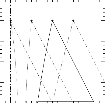
Figure 6.1 Backwards characteristics through several events in the Kerr–Schild metric of a Schwarzschild black

hole. The interval γ

is the domain of dependence of the event Q; the cone deﬁned by γ

and Q is the domain of

determinacy of the interval γ

. The dashed line tracks the event horizon, and the dashed-dotted lines mark some

hypothetical computational boundaries.

their gradients on the boundary. We will encounter various other boundary conditions in

the course of this book.

At this point it is useful to discuss hyperbolic equations in some more detail. The

concept of characteristics leads to the notion of the domain of dependence. For hyperbolic

systems information travels along characteristics. Since no information can travel faster

than the fastest characteristics, the solution at a certain event can only be affected by

those events that lie inside the causal past,orpast cone deﬁned by the fastest ingoing

and outgoing characteristics. In the context of relativity we are quite used to this concept,

since causality demands that an event can only be affected by events in its past light

cone.

For example, consider the wave equation (6.12) for a scalar wave φ that propagates in

a Schwarzschild spacetime expressed in Kerr–Schild coordinates. In Figure 6.1 we plot

several events in this spacetime together with their backward characteristics. Consider the

event Q, whose past characteristics are marked by solid lines. To completely determine

φ(t, r )atQ, we would have to provide initial data φ(0, r)and∂

φ(0, r) inside the past

cone deﬁned by the two backward characteristics, namely on the interval γ

. This is the

domain of dependence of the point Q.

In reverse, for any interval γ on the r -axis, there is a region of the spacetime in which

all events depend only on initial data provided on γ . This region is called the domain of

determinacy.Forγ

in Figure 6.1 the domain of determinacy is the cone deﬁned by γ

and the event Q, bordered by solid lines.

188 Chapter 6 Numerical methods

Suppose we want to obtain a solution to the wave equation (6.12). We will have to

provide initial data on an interval γ that extends from a certain radius r

min

to a radius r

max

at, say, t = 0. If we want to construct the solution only in the domain of determinacy of

γ , then the solution is completely determined by the initial data on γ , and no boundary

conditions are needed. This situation, however, is rarely the case. It is more typical that

we would like to construct the solution in the entire domain between r

min

and r

max

for all

t > 0.

For concreteness, imagine we want to ﬁnd φ in the domain between r

min

/M = 1and

max

/M = 9, marked by the dashed-dotted lines in Figure 6.1. The event Q would still be

completely determined by the initial data, but the event S, for example, would not. One

of its backward characteristics intersects the outer boundary at r

max

/M = 9. The event S

is therefore outside the domain of determinacy of γ , and the solution at S depends on

more information than is provided by the initial data. This missing information now has

to be provided by the boundary conditions. The boundary condition at the outer boundary

max

has to specify the information that propagates along the ingoing characteristic that

originates on the outer boundary. For example, this could be an outgoing-wave boundary

condition which, as the name suggests, insures that no wave (i.e., no information) enters

the domain through the outer boundary.

The situation is different at the inner boundary r

min

. Consider, for example, the event P,

which lies on the boundary r

min

. Since we have chosen r

min

to be inside the event horizon,

both characteristics originate from a larger r, and neither one intersects the boundary r

min

The event P is therefore completely determined by the initial data (and, had we chosen

P at a later time, by the outer boundary condition at r

max

). There is no need to impose a

boundary condition at r

min

, and in fact it would be inconsistent with the equations. This

property will be important when we discuss black hole excision in Chapter 13.1.

Following this general discussion of partial differential equations, we now turn to com-

putational methods that can be used to solve these equations.

6.2 Finite difference methods

Finite difference methods for general applications in computational physics have been

treated in great detail in many references.

Speciﬁc applications to numerical relativity

have been discussed in a few review articles

and many journal articles. Here we provide

a brief introduction that touches on some of the important aspects of the subject.

6.2.1 Representation of functions and derivatives

In a ﬁnite difference approximation a function f (t, x) is represented by values at a discrete

set of points. At the core of ﬁnite difference approximation is therefore a discretization of

e.g., Richtmyer and Morton (1967); Roache (1976); Press et al. (2007).

e.g., Smarr (1979a); Evans et al. (1989).

6.2 Finite difference methods 189

the spacetime, or a numerical grid. Instead of evaluating f at all values of x, for example,

we only consider discrete values x

. As we discuss in more detail in Section 6.2.2,these

gridpoints may reside either at the centers or the vertices of gridcells, but this distinction is

irrelevant for our purposes in this section. The distance between the gridpoints x

is called

the grid spacing x, which in principle may depend on x (or rather x

). For uniform grids,

for which x is constant, we have

= x

+ i x. (6.15)

If the solution depends on time we also discretize the time coordinate, for example as

= t

+ nt, (6.16)

where the superscript n denotes the nth time level and should not be confused with an

exponent. In more than one space dimension the other dimensions are discretized in the

same manner. The result of this is a spacetime lattice, on which all functions can be

evaluated. The ﬁnite difference representation of the function f (t, x), for example, is

= f (t

, x

) + truncation error. (6.17)

Here (and only here) we have explicitly added the “truncation error” as a reminder that

only approaches the correct value of f at t

and x

as the ﬁnite difference solution

converges to the correct solution. We will discuss the ﬁnite difference error in much more

detail below.

Differential equations involve derivatives, so we must next discuss how to represent

derivatives in a ﬁnite difference representation. Consider a partial derivative of f (x) with

respect to x. Assuming that f (x) can be differentiated to sufﬁciently high order and that it

can be represented as a Taylor series, we have

i+1

= f (x

+ x) = f (x

) + x(∂

f )

(x)

(∂

f )

+ O(x

). (6.18)

Solving for (∂

f )

= (∂

f )

we ﬁnd

(∂

f )

i+1

− f

x

O(x). (6.19)

In the limit x → 0 equation (6.19) is just the deﬁnition of the partial derivative, so this

result should not come as a great surprise. The truncation error of this expression is linear

in x, and it turns out that we can do better. Consider the Taylor expansion to the point

i−1

= f (x

− x) = f (x

) − x(∂

f )

(x)

(∂

f )

+ O(x

). (6.20)

Subtracting (6.20) from (6.18)wenowﬁnd

(∂

f )

i+1

− f

i−1

2x

O(x

), (6.21)

190 Chapter 6 Numerical methods

which is second order in x, meaning that the truncation error drops by a factor of four

when we reduce the grid spacing by a factor of 2.

The key point is that we are able to

combine the two Taylor expansions in such a way that the leading order error term cancels

out, leaving us with a higher order representation of the derivative. This cancellation only

works out for uniform grids, when x is independent of x. This is one of the reasons

why many current numerical relativity applications of ﬁnite difference schemes work with

uniform grids.

Exercise 6.4 The ﬁnite difference representation (6.21) being second-order implies

that it should be exact for any arbitrary polynomial up to second order. Verify

that it indeed gives the correct derivative of a polynomial f (x) = a + bx +cx

independently of x and x.

We call equation (6.19)aone-sided derivative, since it uses only neighbors on one side

of x

, and (6.21)acentered derivative. In general, centered derivatives lead to higher order

schemes than one-sided derivatives for the same number of gridpoints. Exercise 6.4 shows

that we can also construct one-sided, higher-order difference schemes, but they will involve

more than two gridpoints.

Exercise 6.5 Construct a second order, one-sided ﬁnite difference approximation

of ∂

f , i.e., generalize equation (6.19), using only neighbors on one side of x

,so

that the truncation error becomes

O(x

). Verify your result by showing that it gives

the exact result for an arbitrary polynomial f (x) = a + bx + cx

, as in exercise 6.4.

Higher-order derivatives can be constructed in a similar fashion. Adding the two Taylor

expansions (6.18) and (6.20) all terms odd in x drop out and we ﬁnd for the second

derivative

(∂

f )

i+1

− 2 f

+ f

i−1

(x)

+ O(x

). (6.22)

This expression is second order because the third order terms in equations (6.18)and

(6.20) cancel out in the addition. An alternative derivation of the second derivative (6.22)

proceeds as follows. First write the ﬁrst derivative at an indermediate grid point x

i+1/2

( f

i+1

− f

)/x and similar at x

i−1/2

. The second derivative at x

is then the derivative of the

derivative, which we can compute from the difference between (∂

f )

i+1/2

and (∂

f )

i−1/2

The result is equation (6.22), and it is second-order accurate because all differences

involved in the derivation were properly centered.

Numerical relativity codes often use ﬁnite-difference representations that are higher

than second order. These can be derived in complete analogy to our above derivation of the

second-order stencils. The key idea is that we want to express the derivative of a function

at a certain grid point, say (∂

f )

, as a linear combination of function values at this and

This is correct only in the limit of small x since for ﬁnite x the higher-order error terms also contribute to the

truncation error.