Baumgarte T., Shapiro S. Numerical Relativity. Solving Einstein’s Equations on the Computer

Подождите немного. Документ загружается.

9.4 Extracting gravitational waveforms 341

where we have used the abbreviation

≡ γ

θθ

φφ

sin

. (9.82)

Exercise 9.6 Show that for an even-parity, l = 2, m = 0 linearized wave represented

by equation (9.48), the coefﬁcients (9.78)–(9.81)aregivenby

220

= 4A

(9.83)

120

= 2rB

(9.84)

=−2A

(9.85)

= (2C − A)

. (9.86)

Hint: Instead of inserting the metric coefﬁcients deﬁned by (9.48) into the quadra-

tures (9.78)–(9.81) and carrying out the integrations, it may be easier to express the

angular dependence in the metric coefﬁcients in terms of spherical harmonics, and

then use their orthogonality relations to ﬁnd the integrals.

We can now combine the coefﬁcients (9.78)–(9.81) to form the gauge-invariant Moncrief

function

r[l(l + 1)k

1lm

+ 4(1 − 2M/r)

2lm

]

l(l + 1)[(l − 1)(l + 2) + 6M/r]

, (9.87)

where the functions

1lm

= K

+l(l + 1)G

+ 2



1 −



r∂

−

1lm



, (9.88)

2lm

2(1 − 2M/r )

−

√

1 − 2M/r

∂



r[K

+l(l + 1)G

]

√

1 − 2M/r



(9.89)

are gauge-invariant themselves. In a Schwarzschild spacetime, the function R

satisﬁes

the famous Zerilli equation

∂

− ∂

∗

+ V

(e)

= 0. (9.90)

Here V

(e)

is the Zerilli potential

(e)

(r) =



1 −



(9.91)

l(l + 1)(l −1)

(l + 2)

+ 6(l − 1)

(l + 2)

+ 36(l − 1)(l + 2)M

r +72M

(

(l − 1)(l + 2)r + 6M

)

Zerilli (1970) and references therein.

342 Chapter 9 Gravitational waves

and r

∗

denotes the tortoise coordinate

∗

= r + 2M ln



− 1



. (9.92)

Exercise 9.7 Revisiting the even-parity, l = 2, m = 0 linearized wave of exercise

9.6, show that the Moncrief function R

is given by

(r∂

A − 6A − 6B + 12C). (9.93)

From the Moncrief functions R

we can determine the asymptotic gravitational wave

amplitudes h

and h

. We postpone displaying these expressions (see equation 9.106)

until after we have introduced the odd-parity (or axial) modes.

Odd-parity (axial) modes

Recall that the only odd-parity spherical harmonics are the magnetic-type vector spherical

harmonics S

and the tensor harmonics S

. Accordingly, the nonangular parts of the

metric cannot have an odd-parity perturbation, and we must have

olm

= 0. (9.94)

The mixed angular-nonangular parts can be expanded in terms of the vector spherical

harmonics S

olm

= V

(t, r)S

(θ,φ) (9.95)

olm

= C

(t, r)S

(θ,φ), (9.96)

and the completely angular part in terms of the tensor spherical harmonics S

olm

=−2r

(t, r)S

(θ,φ). (9.97)

In matrix form, the perturbative matrix then appears as

olm

µν







00−V

/ sin θ V

sin θ S

00−C

/ sin θ C

sin θ S

sym sym r

/ sin θ −r

sin θ

sym sym sym −r

sin θ







, (9.98)

wherewehaveusedequation(D.25) to express S

in terms of the functions X

and W

(see equations D.10 and D.11).

As for the even-parity modes, we can ﬁnd the expansion coefﬁcients V

, C

and

for a given spacetime metric from a surface integration at large radius. Using the

9.4 Extracting gravitational waveforms 343

orthogonality relations in Appendix D we ﬁnd

l(l + 1)



)

∗

d

=−

l(l + 1)



sin θ



(∂

)

∗

rθ

− (∂

)

∗

rφ



d (9.99)

and

=−

(l − 1)l(l + 1)(l + 2)r



)

∗

d

(l − 1)l(l + 1)(l + 2)r



sin θ



−

∗

− γ

θφ

∗



d. (9.100)

We now combine the coefﬁcients C

and D

to form the odd-parity, gauge-invariant

Moncrief function



1 −



∂

). (9.101)

In a Schwarzschild spacetime, Q

satisﬁes the vacuum Regge–Wheeler equation

∂

− ∂

∗

+ V

(o)

= 0, (9.102)

where the Regge–Wheeler potential is

(o)

(r) =



1 −



l(l + 1)

−



. (9.103)

The Moncrief functions Q

are the odd-parity equivalent of the functions R

for even-

parity modes, and we can now discuss how to extract gravitational radiation from these

two functions.

Gravitational wave extraction

We start by splitting the two gravitational wave polarizations h

and h

into even- and

odd-parity parts,

(t, r,θ,φ) = h

(o)

(t, r,θ,φ) + h

(e)

(t, r,θ,φ) (9.104)

(t, r,θ,φ) = h

(o)

(t, r,θ,φ) + h

(e)

(t, r,θ,φ). (9.105)

It then turns out that we can express both parts in terms of the gauge-invariant Moncrief

functions at spatial inﬁnity r →∞. For the even-parity modes we have

(e)

− ih

(e)

∞



l=2



m=−l

)

(l + 2)!

(l − 2)!

(t, r)

−2

(θ,φ), (9.106)

Regge and Wheeler (1957).

344 Chapter 9 Gravitational waves

where

−2

is the s =−2 spin-weighted spherical harmonic (see equation D.9), and for

the odd-parity modes we ﬁnd

(o)

− ih

(o)

=−

∞



l=2



m=−l

)

(l + 2)!

(l − 2)!

(t, r)

−2

(θ,φ). (9.107)

Here the functions q

can be computed from the Moncrief function Q

by integrating

over time,

(t, r) =



−∞



, r)dt



. (9.108)

Using the property (D.6) of spherical harmonics, we can compute the individual even- and

odd-parity polarizations to be

(e)

∞



l=2



+ 2



m=1

Re(R

)



(9.109)

(e)

∞



l=2



m=1



sin θ



(9.110)

(o)

=−

∞



l=2



m=1



sin θ



(9.111)

(o)

∞



l=2



+ 2



m=1

Re(q

)



. (9.112)

We are now ready to use this decomposition to compute the change in energy, angular

momentum and linear momentum of a source due to gravitational radiation. To compute

the energy change, we insert equations (9.109)–(9.112) into equation (9.30) and use the

orthogonality relation for spin-weighted spherical harmonics (D.13)toﬁnd

=−

16π

∞



l=2



m=−l

(l + 2)!

(l − 2)!

(|Q

). (9.113)

Similarly, we can ﬁnd the change in angular momentum from equation (9.35),

=−

16π

∞



l=2



m=−l

(l + 2)!

(l − 2)!

∗

+ R

∗

)

8π

∞



l=2



m=1

(l + 2)!

(l − 2)!

Im(q

∗

+ R

∗

). (9.114)

We could also compute the change in linear momentum from equation (9.36). The result

in terms of Moncrief variables is rather complicated, however, and we refer the reader

elsewhere for the relevant expression.

See Koppitz et al. (2007), equation (3), for the relation.

9.4 Extracting gravitational waveforms 345

0.008

0.006

0.004

0.002

−0.002

−0.004

−0.006

−0.008

−4 −2

024

t − r

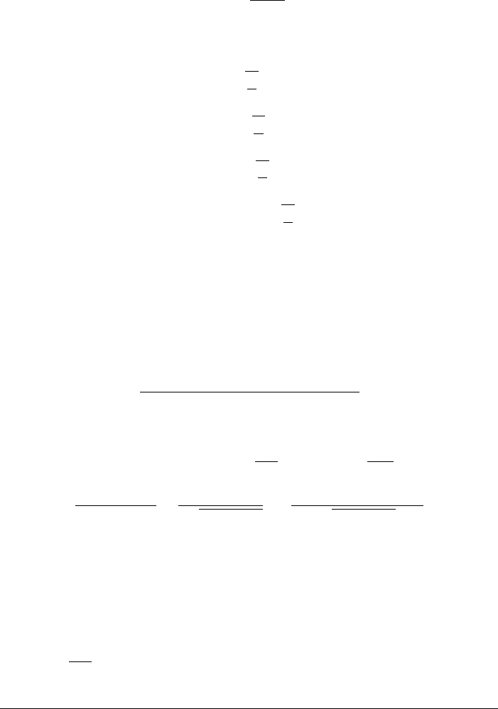
Figure 9.7 The Moncrief function R

at r = 6.0foral = 2, m = 0 linear wave. The solid (black) line denotes

numerical results, and the dashed (red) line is the analytical value given by equation (9.93).

Exercise 9.8 Returning to the even-parity, l = 2, m = 0 linearized wave of exercises

9.6 and 9.7, ﬁnd the wave polarizations h

and h

from equations (9.109)and(9.110)

and compare with the results you would obtain from equations (9.57)and(9.58).

Then compute the radiated energy from equation (9.113) and compare with the result

of exercise 9.5.

It may be useful to illustrate this procedure with a concrete, numerical example. Consider

an even-parity, l = 2, m = 0 linearized wave, as in exercises 9.4 through 9.8. Choose

the function F(x) to have the form of equation (9.56), with amplitude

A = 0.001 and

spatial extend λ = 1 (in arbitrary units). Using this wave to specify the initial data (γ

, K

= 0) in a numerical simulation we now evolve it by adopting the BSSN 3 +1

formalism described in Chapter 11.5. We employ a ﬁnite difference implementation that

is fourth-order accurate in space and second-order in time (cf. Chapter 6.2). We also adopt

geodesic slicing with α = 1andβ

= 0 (Section 4.1), assume equatorial symmetry, and

use a spatial grid of 120 × 120 × 60 grid points in the x, y and z directions, respectively.

Extracting the Moncrief coefﬁcients at a radius of r = 6.0,

we can compute the Moncrief

function R

as a function of time. In Figure 9.7, we show this function together with

its analytical value, which is given by equation (9.93). We could then compute h

from

equation (9.109), but we shall postpone this step until we can compare this procedure with

the Newman–Penrose formalism in Figure 9.8 at the end of the following section.

This is the same gauge as used to express the linearized wave spacetime solutions in equations (9.48)and(9.60), so

we can compare the numerical and analytic values of g

directly. But were we to evolve with a different lapse and

shift we would compare gauge-invariant quantities, like the gauge-invariant Moncrief variables, or the polarization

amplitudes h

and h

This simulation was carried out using a “ﬁsheye” coordinate system that provides radial adaptivity in a simple way (see,

e.g., Campanelli et al. 2006). The grid-spacing in this coordinate system is 

x = 

y = 

z = 0.075, and gravitational

waves are extracted at

r = 4, which corresponds to a physical radius of r = 5.9987.

346 Chapter 9 Gravitational waves

Exercise 9.9 In many problems the dominant modes of gravitational wave emission

are the even l = 2 mass quadrupole modes. Show that in this case the waveform

reduces to



64π

22+

cos 2φ + R

22−

sin 2φ)(1 +cos

θ) +

64π

20∗

sin

16π

21+

cos φ − R

21−

sin φ)sinθ cos θ



, (9.115)



64π

(−R

22+

sin 2φ + R

22−

cos 2φ)cosθ

−

16π

21+

sin φ

A + R

21−

cos φ)sinθ



, (9.116)

where

22+

= 2

√

24 Re(R

), R

22−

=−2

√

24 Im(R

), (9.117)

20∗

= 4

√

, (9.118)

21+

= 2

√

24 Re(R

), R

21−

= 2

√

24 Im(R

). (9.119)

Thus, equations (9.115)and(9.116) are the relativistic generalizations of the weak-

ﬁeld, slow-velocity quadrupole expressions (9.24)and(9.25).

9.4.2 The Newman–Penrose formalism

The 4-dimensional Riemann tensor

(4)

abcd

contains 20 independent components; 10 of

these are absorbed in its trace, the Ricci tensor, and the other 10 in its traceless part, the

Weyl tensor

(4)

abcd

. In the Newman–Penrose formalism,

the 10 independent components

of the Weyl tensor are expressed in terms of ﬁve complex scalars, ψ

,...,ψ

, which are

sometimes called Newman–Penrose scalars and sometimes Weyl scalars. These scalars are

formed by contracting the Weyl tensor with a complex null tetrad. Unfortunately there is

not one unique such null tetrad, and different choices for this tetrad affect the Weyl scalars

and their physical interpretation. One of the conceptional issues in the Newman–Penrose

formalism is therefore the identiﬁcation of a suitable null tetrad.

It is possible to identify

a class of tetrads, called transverse frames, in which the “odd” scalars ψ

and ψ

vanish.

In a subset of these frames, the so-called quasi-Kinnersley frames, we can then interpret

the scalars ψ

and ψ

as measures of the ingoing and outgoing gravitational radiation,

while ψ

represents longitudinal, or “Coulombic” parts of the gravitational ﬁelds, related

to the mass and angular momentum of the spacetime. In this section we are particularly

interested in the Weyl scalar ψ

Newman and Penrose (1962, 1963).

See, for example, Lehner and Moreschi (2007) for a discussion of some of the related issues.

9.4 Extracting gravitational waveforms 347

To construct a null tetrad suitable for our purposes here, we start by choosing two real

vectors l

and k

that are radially outgoing and ingoing null vectors, respectively. We also

construct a complex vector m

from the two spatial vectors that are orthogonal to l

and

in such a way that the only nonvanishing inner products between these 4-vectors are

−l

= 1 = m

, (9.120)

where

is the complex conjugate of m

. We then deﬁne the Weyl scalar ψ

=−

(4)

abcd

, (9.121)

where

(4)

abcd

is the Weyl tensor (1.26).

Exercise 9.10 Show that we may replace the Weyl tensor

(4)

abcd

with the Riemann

tensor

(4)

abcd

in the deﬁnition (9.121) of the Weyl scalar ψ

Some authors adopt a different sign convention in equation (9.121). Further differences

exist in the procedure and conventions for constructing speciﬁc tetrads. For simplicity we

will use a tetrad formed from an orthonormal spherical polar basis according to

√



+ e



√



− e



√



+ ie



√



− ie



(9.122)

Exercise 9.11 Verify that the tetrad (9.122) satisﬁes the orthogonality relations

(9.120).

We can now verify that ψ

indeed provides a measure of outgoing radiation. According

to exercise 9.10 we may contract the Riemann tensor

(4)

abcd

with k

and

to compute

in equation (9.121), which yields

=−



(4)

− 2i

(4)

− 2

(4)

+ 2i

(4)

−

(4)

+ 2i

(4)

+ 2

(4)

− 2i

(4)

−

(4)



. (9.123)

To linear order in small deviations from ﬂat spacetime the Riemann tensor reduces to

(4)

abcd

(

∂

+ ∂

∂

− ∂

∂

− ∂

∂

)

. (9.124)

In the TT gauge, the only nonvanishing components of a radially propagating wave are

the transverse, angular components h

=−h

and h

= h

. As in equations (9.57)

We may always replace the Weyl tensor with the Riemann tensor in vacuum, where they are identical, but in the

deﬁnition of ψ

we may make this replacement everywhere.

348 Chapter 9 Gravitational waves

and (9.58), we may identify the former with h

and the latter with h

. Since all terms

in equation (9.123) have exactly two angular indices, the only nonzero terms in equa-

tion (9.124) are those for which these two angular indices appear in the metric perturbation

, and the t and r indices appear in the partial derivatives. For example, the ﬁrst term in

equation (9.123) reduces to

(4)

=−

∂

=−

. (9.125)

For an outgoing wave at large r we know that h

(t, r,θ,φ) = h

(t − r,θ,φ), hence

∂

=−∂

, so that we can express radial derivatives in terms of time derivatives.

Collecting all terms, we then ﬁnd

− i

. (9.126)

Exercise 9.12 Retrace the steps outlined above to show that for a purely ingoing

wave the Weyl scalar ψ

vanishes.

As claimed above, the Weyl scalar ψ

thus provides a measure of outgoing gravitational

radiation. We can therefore use ψ

to compute gravitational wave signals, as well as the

radiated energy and angular and linear momentum. Before proceeding to do that, however,

we point out a computational issue.

Computing ψ

involves the 4-dimensional Riemann tensor

(4)

abcd

. Many numerical

simulations, however, employ a 3+1 formalism that is based on working with 3-dimensional

spatial quantities. Before we can compute ψ

, then, we ﬁrst have to construct

(4)

abcd

from

these spatial quantities. In principle, we may do this by reversing the steps in Chapter 2.5 and

using the Gauss, Codazzi and Ricci equations. More speciﬁcally, we can ﬁnd

(4)

abcd

from

equation (2.61), which expresses

(4)

abcd

in terms of its spatial and normal projections. We

can then substitute equations (2.68), (2.73) and (2.103), which relate these projections to

purely spatial quantities. Under some circumstances, this procedure simpliﬁes signiﬁcantly.

If we may assume that in some asymptotically ﬂat regime the deviations of the lapse

from unity and the shift from zero are at most as large as the Riemann tensor itself, then we

may approximate the normal vector in equations (2.73) and (2.103)asn

 δ

. Restricting

equations (2.68), (2.73) and (2.103) to spatial indices, and assuming a vacuum, then yields

(4)

ijkl

= R

ijkl

+ 2K

i[k

l] j

(4)

0 jkl

= 2∂

l] j

+ 2K

m[k



l] j

(4)

0 j0l

= R

− K

+ KK

(9.127)

The above expressions for

(4)

abcd

maythenbeusedinequation(9.121)toevaluateψ

large r in the wave zone on each time slice in a 3 + 1 numerical simulation.

This expression again depends on conventions. It sometimes appears with the opposite sign in the literature, related

to the sign convention in equation (9.121), or with a factor of 1/2, if a different normalization is used in the tetrad

deﬁnition (9.122).

9.4 Extracting gravitational waveforms 349

Exercise 9.13 Some authors deﬁne the ingoing null tetrad vector k

in equa-

tion (9.122) in terms of the normal vector n

plus a purely spatial, radially outward

pointing vector v

, e.g.,

√

(

− v

)

. (9.128)

Show that with this deﬁnition, ψ

can be expressed as

=−



(4)

pqrs

− 2γ

(4)

pqrs

+γ

(4)

pqrs



, (9.129)

into which we can then substitute equations (2.68), (2.73)and(2.143) for the pro-

jections of

(4)

abcd

We now return to computing the gravitational wave emission from ψ

. We can ﬁnd

the gravitational waveforms h

and h

by integrating the real and imaginary parts of

equation (9.126) twice. Knowing h

and h

, we can then compute the radiated energy and

momenta by substituting into equations (9.30), (9.35) and (9.36). In particular, we ﬁnd

=−

= lim

r→∞

16π



d





−∞





(9.130)

for the gravitational wave luminosity and corresponding loss of energy from the source,

= lim

r→∞

16π



d Re







−∞





∂



−∞







−∞



∗





(9.131)

for the angular momentum loss, and

= lim

r→∞

−

16π



d





−∞





(9.132)

for the linear momentum loss.

For many applications it is useful to decompose ψ

into s =−2 spin-weighted spherical

harmonics

(t, r,θ,φ) =

∞



l=2



m=−l

(t, r)

−2

(θ,φ) (9.133)

(see Appendix D). Using the orthogonality relation (D.13) we can ﬁnd the expansion

coefﬁcients ψ

from



d

−2

∗

. (9.134)

Exercise 9.14 Compare equation (9.126) with equations (9.106)and(9.107)to

show that ψ

is related to the Moncrief variables R

and Q

)

(l + 2)!

(l − 2)!

(

− i

). (9.135)

350 Chapter 9 Gravitational waves

In terms of the coefﬁcients ψ

, the gravitational wave luminosity (9.130)is

=−

= lim

r→∞

16π

∞



l=2



m=−l





−∞





, (9.136)

while the loss of angular momentum due to gravitational waves, equation (9.131), becomes

= lim

r→∞

16π

∞



l=2



m=−l

m Im







−∞







−∞







−∞



lm∗





. (9.137)

For some purposes it is useful to introduce real functions A

and B

whose second time

derivative equals the real and imaginary parts of ψ

lm∗

− i

. (9.138)

In terms of these, the loss of energy and angular momentum due to waves become

=−

= lim

r→∞

16π

∞



l=2



m=−l

(

) (9.139)

and

= lim

r→∞

16π

∞



l=2



m=−l

−

). (9.140)

Similarly we can express the loss of linear momentum (9.132) in terms of these coefﬁcients,

but as in the Moncrief formalism that leads to a rather lengthy expression that we shall

omit.

Before closing this chapter we return to the numerical example at the end of Section

9.4.1, namely the l = 2, m = 0 even-parity linearized wave. We evolve the same initial data

with the same numerical code as described there, but instead of extracting the Moncrief

variable R

(see Figure 9.7) we now compute the Weyl scalar ψ

at a point (r,θ,φ) =

(6.0, 0.79, 0.52) (see footnote 45 above).We compare the numerical values with analytical

expressions in the left panels of Figure 9.8. In the right panels we also graph the analytic

gravitational waveforms for both polarizations, as well as the corresponding numerical

waveforms using both the Moncrief formalism (computed from equation 9.109) and the

Newman–Penrose formalism (computed from equation 9.126).

Figure 9.8 demonstrates that, for this particular example, the Moncrief formalism leads

to a better agreement with the analytical results than the Newman–Penrose formalism (even

though both converge to the analytical results as the numerical resolution is increased

This difference can be attributed to two factors. One difference between the two approaches

See, e.g., Ruiz et al. (2008a).

We also point out that while h

computed in Figure 9.8 from the Newman–Penrose formalism is not as close to the

analytic value of zero as the value computed by the Moncrief formalism, it is still more than an order of magnitude

below the amplitude of the dominant h

polarization amplitude for the adopted resolution.