Bielajew A.F. Fundamentals of the Monte Carlo method for neutral and charged particle transport

Подождите немного. Документ загружается.

14.2. PRESTA 231

terminated, was chosen to be 1% of the starting energy. The only exception was 10 keV,

where the endpoint energy was 1 keV. We note that both hzi

and hri

exhibit step-

size independence. Even more remarkable is the fact that the minor step-size dependence

exhibited by hri

, shown in ﬁg. 14.21, has vanished. This improvement appears to be

fortuitous resulting form cancellations of second-order eﬀects. More research is needed to

study the theories concerning lateral displacements.

14.2.6 PRESTA’s boundary crossing algorithm

The ﬁnal element of PRESTA is the boundary crossing algorithm. This part of the algorithm

tries to resolve two irreconcilable facts: that electron transport must take place across bound-

aries of arbitrary shape and orientation, and that the Moli`ere multiple scattering theory is

invalid in this context.

If computing speed did not matter, the solution would be obvious—use as small a step-size

as possible within the constraints of the theory. With this method, a great majority of the

transport steps would take place far removed from boundaries and the underlying theory

would only be “abused” for that small minority of steps when the transport takes place in

the direct vicinity of boundaries. This would also solve any problems associated with the

omission of lateral translation and path-length correction. However, with the inclusion of a

reliable path-length correction and lateral correlation algorithm, we have seen that we may

simulate electron transport with very large steps in inﬁnite media. For computing eﬃciency,

we wish to use these large steps as often as possible.

Consider what happens as a particle approaches a boundary in the PRESTA algorithm.

First we interrogate the geometry routines of the transport code and ﬁnd out the closest

distance to any boundary. As well as any other restrictions on electron step-size, we restrict

the electron step-size, (total, including path-length curvature) to the closest distance to any

boundary. We choose to restrict the total step-size so that no part of the electron path could

occur across any boundaries. We then transport the particle, apply path-length corrections,

the lateral correlation algorithm, and perform any “scoring” we wish to do. We then repeat

the process.

At some point this process must stop, else we encounter a form of Xeno’s paradox. We will

never reach the boundary! We choose a minimum step-size which stops this sort of step-size

truncation. We call this minimum step-size t

min

. If a particle’s step-size is restricted to t

min

we are in the vicinity of a boundary. The particle may or may not cross it. At this point,

to avoid ambiguities, the lateral correlation algorithm is switched oﬀ, whether or not the

particle actually crosses the boundary. If we eventually cross the boundary, we transport

the particle with the same sort of algorithm. We start with a step t

min

.Wethenletthe

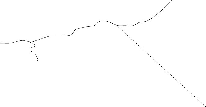
above algorithm take over. This process is illustrated in ﬁg. 14.24. This example is for a 10

MeV electron incident normally upon a 1 cm slab of water. The ﬁrst step is t

min

in length.

232 CHAPTER 14. ELECTRON STEP-SIZE ARTEFACTS AND PRESTA

Figure 14.24: Boundary crossing algorithm example: A 10 MeV electron enters a 1 cm slab

of water from the left in the normal direction. The ﬁrst step is t

min

in length. Since the

position here is less than t

min

away from the boundary, the next step is length t

min

as well.

The next 4 steps are approximately 2t

min

,4t

min

,8t

min

,and16t

min

in length, respectively.

Finally, the transport begins to be inﬂuenced by the other boundary, and the steps are

shortened accordingly. The electron leaves the slab in 3 more steps.

Since the position at this point is less than t

min

away from the boundary (owing to path

curvature), the next step is length t

min

as well. The next 4 steps are approximately 2t

min

,8t

min

,and16t

min

in length, respectively. Finally, the electron begins to “see” the

other boundary, shortens its steps accordingly. For example, the total curved path “a” in

the ﬁgure is associated with the transport step “b”. The distance “a” is the distance to the

closest boundary.

Finally, what choice should be made for t

min

? One could choose t

min

= t

min

, the minimum

step-size constraint of the Moli`ere theory. Although this option is available to the PRESTA

user, practice has shown it to be too conservative. Larger transport steps may be used

in the vicinity of boundaries. The following choice, the default setting for t

min

, has been

found to be be a good practical choice, allowing both accurate calculation and computing

eﬃciency: Choose t

min

to equal t

max

for the minimum energy electron in the problem (as

set by transport cut-oﬀ limits). Then scale the energy-dependent parts of the equation for

min

accordingly, for higher energy electrons. The reader is referred to ref. [BR87] for the

mathematical details. As an example, we return to the “air tube” calculation of ﬁg. 14.16.

In that ﬁgure, the choice of “blcmin”, the variable in PRESTA which controls the boundary

crossing algorithm and which is closely related to t

min

, was set to 1.989. This causes t

min

to be equal to t

max

for 2 keV electrons. A transport cut-oﬀ of 2 keV is appropriate in this

simulation because electrons with this energy have a range which is a fraction of the diameter

of the tube. In most practical problems, if one chooses the transport cut-oﬀ realistically,

PRESTA’s default selection for t

min

produces accurate results. Again, the reader is referred

to the PRESTA documentation [BR87] for further discussion.

14.2. PRESTA 233

PRESTA, as the name implies, was designed to calculate quickly as well as accurately, since

it wastes little time taking small transport steps in regions where it has no need to. There

is no space to go into further discussion about this although there is a brief discussion in

Chapter 17. Again, the reader is referred elsewhere [BR87]. Typical timing studies have

shown that PRESTA, in its standard conﬁguration, executes as quickly, and sometimes much

more quickly, then EGS with ESTEPE set so as to produce accurate results. For problems

with a ﬁne mesh of boundaries, for example a depth-dose curve with a r

/40 mesh, the timing

is about the same. For other problems, with few boundaries, the gain in speed is about a

factor of 5.

14.2.7 Caveat Emptor

It would leave the reader with a mistaken impression if the chapter was terminated at this

point. PRESTA has demonstrated that step-size dependence of calculated results has been

eliminated in many cases and that computing time can be economized as well. By under-

standing the elements of condensed-history electron transport, some problems have been

solved. Calculational techniques that isolate the eﬀects of various constituents of the elec-

tron transport algorithm have been developed and used to prove their step-size independence.

However, PRESTA is not the ﬁnal answer because it does not solve all step-size dependence

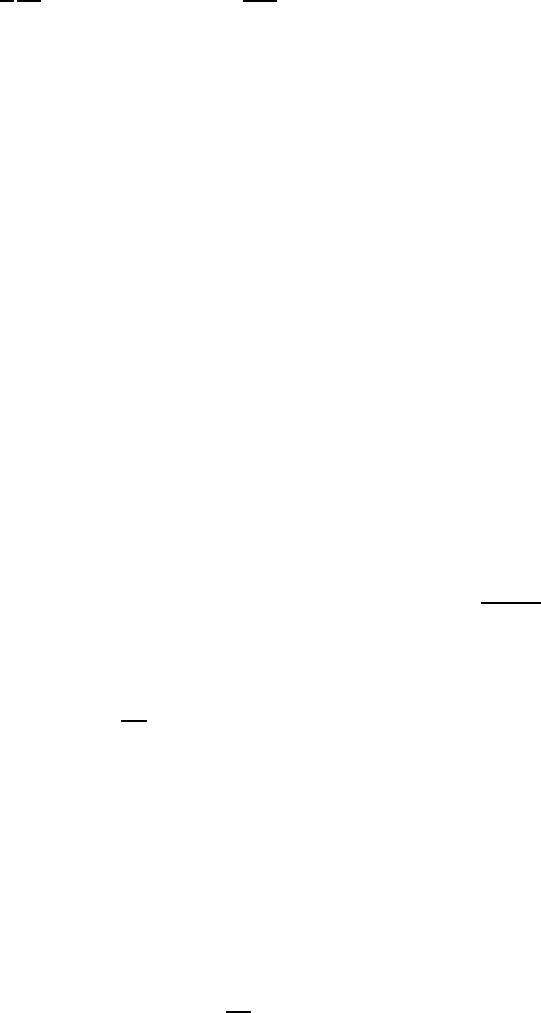
problems, in particular, backscattering. This is demonstrated by the example shown in

ﬁg. 14.25. In this example, 1.0 MeV electrons were incident normally on a semi-inﬁnite

slab of water. The electron transport was performed in the CSDA approximation. That is,

no δ-rays or bremsstrahlung γ’s were set in motion and the unrestricted collision stopping

power was used. The ratio of backscattered kinetic energy to incident kinetic energy was

calculated. The default EGS calculation (with ESTEPE control) is shown to have a large

step-size dependence. The PRESTA calculation is much improved but still exhibits some

residual dependence on step-size.

In general, problems that depend strongly on backscatter will exhibit a step-size dependence,

although the severity is much reduced when one uses PRESTA. We may speculate on the

reason for the existence of the remaining step-size dependence. Recall that the path-length

correction, which relates the straight-line path length, s,andt, the curved path-length of

the transport step, really calculates only an average value. That is, given t,thevalueofs is

predetermined and unique. It is really a distributed quantity and should be correlated to the

multiple scattering angle of the step. In other words, we expect the distribution to be peaked

in the backward direction if Θ = π andpeakedintheforwarddirectionifΘ=0. Tothis

date, distributions of this sort which are accurate for large angle scattering are unknown. If

they are discovered they may cure PRESTA’s remaining step-size dependence.

234 CHAPTER 14. ELECTRON STEP-SIZE ARTEFACTS AND PRESTA

Figure 14.25: Fractional energy backscattered from a semi-inﬁnite slab of water with 1.0 MeV

electrons incident normally. The electron transport was performed in the CSDA approxima-

tion. (No δ-rays or γ’s were set in motion). The default EGS and PRESTA calculations are

contrasted. There is still evidence of step-size dependence in the PRESTA calculation.

Bibliography

[Ber63] M. J. Berger. Monte Carlo Calculation of the penetration and diﬀusion of fast

charged particles. Methods in Comput. Phys., 1:135 – 215, 1963.

[Bet53] H. A. Bethe. Moli`ere’s theory of multiple scattering. Phys. Rev., 89:1256 – 1266,

1953.

[BR87] A. F. Bielajew and D. W. O. Rogers. PRESTA: The Parameter Reduced Electron-

Step Transport Algorithm for electron Monte Carlo transport. Nuclear Instruments

and Methods, B18:165 – 181, 1987.

[BRN85] A. F. Bielajew, D. W. O. Rogers, and A. E. Nahum. Monte Carlo simulation of

ion chamber response to

Co – Resolution of anomalies associated with interfaces,.

Phys. Med. Biol., 30:419 – 428, 1985.

[BS83] M. J. Berger and S. M. Seltzer. Stopping power and ranges of electrons and

positrons. NBS Report NBSIR 82-2550-A (second edition), 1983.

[Eyg48] L. Eyges. Multiple scattering with energy loss. Phys. Rev., 74:1534, 1948.

[Fan54] U. Fano. Note on the Bragg-Gray cavity principle for measuring energy dissipation.

Radiat. Res., 1:237 – 240, 1954.

[GS40a] S. A. Goudsmit and J. L. Saunderson. Multiple scattering of electrons. Phys.

Rev., 57:24 – 29, 1940.

[GS40b] S. A. Goudsmit and J. L. Saunderson. Multiple scattering of electrons. II. Phys.

Rev., 58:36 – 42, 1940.

[HW55] D. F. Hebbard and R. P. Wilson. The eﬀect of multiple scattering on electron

energy loss distribution. Aust. J. Phys., 8:90 –, 1955.

[Lew50] H. W. Lewis. Multiple scattering in an inﬁnite medium. Phys. Rev., 78:526 – 529,

1950.

[Mol47] G. Z. Moli`ere. Theorie der Streuung schneller geladener Teilchen. I. Einzelstreuung

am abgeschirmten Coulomb-Field. Z. Naturforsch, 2a:133 – 145, 1947.

235

236 BIBLIOGRAPHY

[Mol48] G. Z. Moli`ere. Theorie der Streuung schneller geladener Teilchen. II. Mehrfach-

und Vielfachstreuung. Z. Naturforsch, 3a:78 – 97, 1948.

[NHR85] W. R. Nelson, H. Hirayama, and D. W. O. Rogers. The EGS4 Code System.

Report SLAC–265, Stanford Linear Accelerator Center, Stanford, Calif, 1985.

[RBN85] D. W. O. Rogers, A. F. Bielajew, and A. E. Nahum. Ion chamber response and

wall

correction factors in a

Co beam by Monte Carlo simulation. Phys. Med.

Biol., 30:429 – 443, 1985.

[Rog84] D. W. O. Rogers. Low energy electron transport with EGS. Nucl. Inst. Meth.,

227:535 – 548, 1984.

[SA55] L. V. Spencer and F. H. Attix. A theory of cavity ionization. Radiat. Res., 3:239

– 254, 1955.

[Yan51] C. N. Yang. Actual path length of electrons in foils. Phys. Rev, 84:599 – 600,

1951.

Problems

Chapter 15

Advanced electron transport

algorithms

In this chapter we consider the transport of electrons in a condensed history Class II

scheme [Ber63]. That is to say, the bremsstrahlung processes that result in the creation of

photons above an energy threshold E

, and Møller knock-on electrons set in motion above

an energy threshold E

, are treated discretely by creation and transport. Sub-threshold

processes are accounted for in a continuous slowing down approximation (CSDA) model.

For further description of the Class II scheme the reader is encouraged to read Berger’s

article [Ber63] who coined the terminology and gave a full description and motivation for

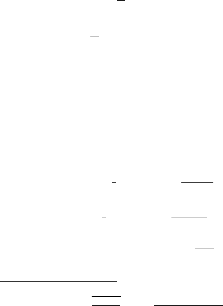
the classiﬁcation scheme. Figure 15.1 gives a graphical description of the transport.

Figure 15.1: This is a depiction of a complete electron history showing elastic scattering,

creation of bremsstrahlung above the E

threshold, the setting in motion of a knock-on

electron above the E

threshold and absorption of the primary and knock-on electrons.

237

238 CHAPTER 15. ADVANCED ELECTRON TRANSPORT ALGORITHMS

The electron transport processes between the particle creation, absorption vertices is gov-

erned by the Boltzmann transport equation as formulated by Larsen [Lar92]:

∂

∂t

Ω ·

∇ + σ

(E) −

∂

∂E

L(E)

ψ(~x,

Ω,E,t)=

4π

dΩ

(

Ω ·

Ω

,E)ψ(~x,

Ω

,E,t) , (15.1)

where ~x is the position,

Ω is a unit vector indicating the direction of the electron, E is the

energy of the electron and t is time. σ

(

Ω ·

Ω

,E) is the macroscopic diﬀerential scattering

cross section,

(E)=

4π

dΩ

(

Ω ·

Ω

,E) (15.2)

is the total macroscopic cross section (probability per unit length), L(E) is the restricted

stopping power appropriate for bremsstrahlung photon creation and Møller electrons beneath

their respective thresholds E

and E

, v is the electron speed and ψ(~x,

Ω,E,t)d~x dΩ dE is

the probability of there being an electron in d~x about ~x,indΩabout

ΩandindE about E

at time t. The boundary condition to be applied to each segment in Figure 15.1 is:

ψ(~x,

Ω,E,0) = δ(~x)δ(ˆz −

Ω)δ(E

− E) , (15.3)

where the start of each segment is translated to the origin and rotated to point in the z-

direction. (ˆz is a unit vector pointing along the z-axis.) The energy at the start of the n-th

segment is E

For our considerations within the CSDA model, we note that E and t can be related since

the pathlength, s,

s = vt =

L(E

)

, (15.4)

permitting a slight simpliﬁcation of Eq. 15.1:

∂

∂s

Ω ·

∇ + σ

(E)

ψ(~x,

Ω,s)=

4π

dΩ

(

Ω ·

Ω

,E)ψ(~x,

Ω

,s) . (15.5)

The cross section still depends on E which may be calculated from Eq. 15.4.

Lewis [Lew50] has presented a “formal” solution to Eq.15.5. By assuming that ψ can be

written in an expansion in spherical harmonics,

ψ(~x,

Ω,s)=

(~x, s)Y

(

Ω) , (15.6)

one ﬁnds that

∂

∂s

+ κ

(~x, s)=−

λµ

∇ψ

λµ

(~x, s) ·

λµ

, (15.7)

where

(E)=

4π

dΩ

(

Ω ·

Ω

,E)[1 − P

(

Ω ·

Ω

)] , (15.8)

239

and

λµ

4π

dΩ Y

∗

(

Ω)

Ω Y

λµ

(

Ω) . (15.9)

If one considers angular distribution only, then one may integrate over all ~x in Eq. 15.7

giving:

∂

∂s

+ κ

(s)=0, (15.10)

resulting in the solution derived by Goudsmit and Saunderson [GS40a, GS40b]:

ψ(

Ω,s)=

4π

(2l +1)P

(ˆz ·

Ω) exp



−

(E)



. (15.11)

Eq. 15.7 represents a complete formal solution of the Class II CSDA electron transport

problem but it has never been solved exactly. However, Eq. 15.7 may be employed to

extract important information regarding the moments of the distributions. Employing the

deﬁnition,

(s)=exp



−

(E)



, (15.12)

Lewis [Lew50] has shown the moments hzi, hz cos Θi,andhx

+ y

i to be:

hzi =

) , (15.13)

hz cos Θi =

(s)

1+2k

)

, (15.14)

and

+ y

i =

)

1 − k

)

. (15.15)

It can also be shown using Lewis’s methods that

i =

)

1+2k

)

, (15.16)

and

+ y

+ z

i =2

)

, (15.17)

which gives the radial coordinate after the total transport distance, s. Note that there was an

error

in Lewis’s paper where the factor 1/3 was missing from his version of hz cos Θi.Inthe

The correction of Lewis’s Eq. 26 is:

4π(2l +1)

(s)

l−1

)+(l +1)k

l+1

)

The reader should consult Lewis’s paper [Lew50] for the deﬁnition of the H-functions.

240 CHAPTER 15. ADVANCED ELECTRON TRANSPORT ALGORITHMS

limit that s −→ 0, one recovers from Eqs. 15.14 and 15.16 the results lim

s−→ 0

hz cos Θi = s

and lim

s−→ 0

i = s

which are not obtained without correcting the error as described in the

footnote. Similar results for the moments have been derived recently by Kawrakow [Kaw96a]

using a statistical approach.

Before leaving this introductory section it warrants repeating that these equations are all “ex-

act” within the CSDA model and are independent of the form of the elastic scattering cross

section. It should also be emphasized that Larsen analysis [Lar92] proves that the condensed

history always gets the correct answer (consistent with the validity of the elastic scattering

cross section) in the limit of small step-size providing that the “exact” Goudsmit-Saunderson

multiple-scattering formalism is employed (and that its numerical stability problems at small

step-size can be solved). Larsen analysis also draws some conclusions about the underlying

Monte Carlo transport mechanisms and how they relate to convergence of results to the cor-

rect answer. Some Monte Carlo techniques can be expected to be less step-size dependent

than others and converge to the correct answer more eﬃciently, using larger steps.

The ultimate goal of a Monte Carlo transport algorithm should be to make electron con-

densed history calculations as stable as possible with respect to step-size. That is, for a

broad range of applications there should be step-size independence of the result. Hence, it

would be most eﬃcient to use steps as large as possible and not be subject to calculation

errors. While we have not yet achieved this goal, we have made much progress towards it

and describe some of this progress in a later section.

15.1 What does condensed history Monte Carlo do?

Monte Carlo calculations attempt to solve Eq. 15.5 iteratively by breaking up the transport

between discrete interaction vertices, as depicted in Figure 15.2. The ﬁrst factor determining

the electron step-size distance is the distance to a discrete interaction. These distances are

stochastic and characterized by an exponential distribution. Further subdivision schemes

may be employed and these can be classiﬁed as numeric, physics’ or boundary step-size

constraints.

15.1.1 Numerics’ step-size constraints

A geometric restriction, say s ≤ s

max

may be used.A geometric restriction of this form was

introduced by Rogers [Rog84b] in the EGS Monte Carlo code [NHR85, BHNR94]. This has

application in graphical displays of Monte Carlo histories. One wants the electron tracks to

have smooth lines and so the individual pathlengths should be of the order of the resolution

size of the graphics display. Otherwise, the tracks look artiﬁcially jagged, as they do in

Figure 15.2. Of course, there are some real sharp bends in the electron tracks associated

with large angle elastic scattering, but these are usually infrequent. One can predict the