Birge J.R., Louveaux F. Introduction to Stochastic Programming

Подождите немного. Документ загружается.

354 8 Evaluating and Approximating Expectations

This form of the L -shaped method follows the same steps as the standard L -

shaped method, except that we add an extra check with the upper bound to deter-

mine the stopping conditions. We also describe the calculation of Q

somewhat

generally to allow for more general types of approximating distributions and ap-

proximating recourse functions, Q

,ξ) .

Example 2

Consider Example 1 from Chapter 5,where:

Q(x,



−x if x ≤

x −

if x >

(3.6)

x = 0,and 0≤ x ≤ 10 . Instead of a discrete distribution on ξ , however, assume

that ξ is uniformly distributed on [0,5] . For the bounding approximation, we use

the Jensen lower bound and Edmundson-Madanskyupper bound for Q

and Q

respectively. We use the reﬁnement procedure to split the cell that contributes most

to the difference between Q

and Q

. We split this cell at the intersection of the

supports from the two extreme points of this cell (here, interval).

The sequence of iterations is as follows.

Iteration 1:

Here, x

= 0.Find Q

(0)=Q(0,

= 2.5)=2.5. E

= −

∂

(0,2.5)=−(− 1)

and e

= −

∂

(0,2.5)(h = 2.5)=−(−1)(2.5)=2.5.Addthecut:

≥ 2.5 −x . (3.7)

Iteration 2:

Here, x

= 10 ,

= −7.5, but Q

(10)=Q(10,

= 2.5)=7.5 . At this

point, the subgradient of Q

(10) is 1 . E

= −

∂

(10,2.5)=−1, and e

−

∂

(0,2.5)(h = 2.5)=−(1)(2.5)=−2.5.Addthecut:

≥−2.5 + x . (3.8)

Iteration 3:

Here, x

= 2.5,

= 0, Q

(2.5)=Q(2.5,

= 2.5)=0 . Hence we meet the

condition for optimality of the ﬁrst lower bounding approximation. Now, go to

Step 4 and consider the ﬁrst upper bounding approximation with equal weights of

0.5on

= 0and

= 5 . In this case, Q

(2.5)=0.5 ∗(Q(2.5,0)+Q(2.5,5)) =

2.5 . Thus, we must reﬁne the approximation. Using the subgradient of −1at

= 0

and 1 and

= 5 , split at c

∗

= 2.5.

8.3 Using Bounds in Algorithms 355

The new lower bounding approximation has equal weights of 0.5on

1.25 and

= 3.75 . In this case, Q

(2.5)=0.5 ∗(Q(2.5,1.25)+Q(2.5,3.75)) =

1.25 . Now, we add the cut E

= 0.5(−

∂

Q(2.5,1.25) −

∂

Q(2.5,3.75)) = 0and

= 0.5(−

∂

Q(2.5,1.25)(1.25)−

∂

Q(2.5,3.75)(3.75)) = (0.5)(−1.25+3.75)=

1.25 . Thus, we add the cut:

≥ 1.25 . (3.9)

Iteration 4:

Here, keep x

= x

= 2.5 (although other optima are possible) and

= 1.25 .

Again, Q

(2.5)=1.25 , so proceed to Step 4.

Checking the upper bound, we ﬁnd that the upper bound places equal weights on

the endpoints of each interval, [0,2.5] and [2.5, 5] . Thus,

(2.5)=0.5 ∗(Q(2.5,2.5)) + (0.25) ∗(Q(2.5,0)+Q(2.5, 5)) = 1.25 , and

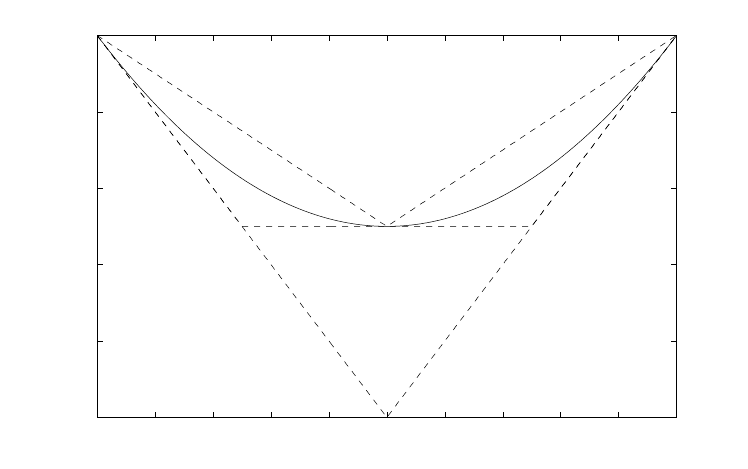
(2.5) . Stop with an optimal solution.

The steps are illustrated in Figure 4. We show the true Q(x) as a solid line,

with dashed lines representing the approximations (lower and upper). Note that the

method may not have converged as quickly if we had chosen some point other than

= x

= 2.5 . The upper and lower bounds meet at this point, because we chose

the division precisely at the link between the linear pieces of the recourse function

Q(x,·) .

0 0.5 1 1.5 2 2.5 3 3.5 4 4.5 5

0.5

1.5

2.5

Fig. 4 Example of L -shaped method with sequential approximation.

356 8 Evaluating and Approximating Expectations

Bounds with generalized programming

In generalized linear programming, the same types of procedures can be applied.

The difference is that because the generalized programming method uses inner lin-

earization instead of outer linearization, the bounds used should be upper bounds.

We would thus substitute

for

in (5.6.6). The same steps are followed again

with

until optimality relative to

is achieved. At this point, as in Step 4

of the L -shaped method with sequential bounding approximations, overall conver-

gence is tested by solving (5.6.10) with a lower bounding

in place of

.Ifthis

value is again non-negative, then the procedure stops. If not, reﬁnement is made un-

til a new upper bounding column is generated or no solution of (5.6.10)isnegative

for a lower bounding approximation.

As stated in Chapter 5, generalized programming is most useful if the recourse

function,

(

) , is separable in the components of

. The separable upper bound-

ing procedure is a natural use for this approach. A separable lower bound can be

obtained by using a supporting hyperplane. This leads to the Jensen lower bound.

This generalized programming approach applies most directly when a single ba-

sis separable approximation is used. With the convex hull operation, we would still

have the problem of evaluating this function. This difﬁculty is, however, overcome

by dualizing the problem. In this case, we suppose that the original problem using a

set D of bases is to ﬁnd x ∈ℜ

∈ ℜ

min c

x + co{

,D ∈ D}(

) (3.10)

s. t. Ax = b ,

Tx−

= 0 ,

x ≥ 0 .

The main result is the following theorem. Recall the conjugate function deﬁned in

Section 2.10.

Theorem 3. A dual program to (3.10) is to ﬁnd

∈ ℜ

max

b −sup{

∗

,D ∈ D}(−

) (3.11)

s. t.

A +

T ≤ c

where

∗

is the conjugate function and (3.10) and (3.11) have equal optimal val-

ues.

Proof:Let

(

)=co{

,D ∈D }(

) . Then a dual to (3.10) (see, e.g., Geoffrion

[1971], Rockafellar [1974]) is

max

{ inf

x≥0,

x +

(

(b −Ax)+

(

−Tx)]} ,

which is equivalently

8.4 Bounds in Chance-Constrained Problems 357

max

{ inf

x≥0,

[(c

−

A −

T)x +

(b) −(−

−

(

))]}

= max

A+

T≤c

{

b −

∗

(−

)} . (3.12)

Problem (3.12) immediately gives (3.11) because (co{

,D ∈ D}(

))

∗

(−

)

= sup{

∗

,D ∈ D}(−

) (Rockafellar [1969, Theorem 16.5]).

Problem (3.11) only involves ﬁnding the supremum of convex functions, which

is again a convex function. The main difﬁculty is in ﬁnding expressions for the

∗

These are, however, relatively straightforward to evaluate (Exercise 2). They can be

used in a variety of optimization procedures, but the objective is nondifferentiable.

In Birge and Wets [1989], this difﬁculty is overcome by making each

∗

alower

bound on some parameter that replaces sup{

∗

,D ∈D } in the objective.

The main reﬁnement choice in the separable optimization procedure using (3.11)

is to determine how to update the set D . Choices of bases that are optimal for

and then

for increasing values of

appear to give a rich set D as

in Birge and Wets [1989]. Any sense of optimal reﬁnements or basis choice is,

however, an open question.

Exercises

1. Consider Example 2 where we redeﬁne Q as

Q(x,ξ)=



2(ξ −x) if x ≤ ξ ,

x −ξ if x > ξ ,

with ξ uniformly distributed on [0,5] , c

x = 0,and 0≤ x ≤ 10 . Follow the

L -shaped sequential approximation method until achieving a solution with two

signiﬁcant digits of accuracy.

2. Find

∗

(−

) and

∂Ψ

∗

(−

) . A useful set may be

(p)={y | P

(y)

−

≤

p ≤ P

(y)}.

3. Use the dualization procedure to solve a stochastic linear program with c

x = x ,

0 ≤ x ≤1 , and the recourse function in Example 1.

8.4 Bounds in Chance-Constrained Problems

Our procedures have so far concentrated on methods for recourse problems as we

have throughout this book. In many cases, of course, probabilistic constraints may

also be in the formulation or may be the critical part of the model. The basic results

are aimed at ﬁnding some inequalities

Ax ≥

h (or, perhaps, nonlinear inequali-

ties) that imply that P{Ax ≥ h}≥

. In Section 3.2, we found some deterministic

358 8 Evaluating and Approximating Expectations

equivalents for speciﬁc forms of the distribution, but these are not always available.

In these cases, it is useful to have upper and lower bounds on P{Ax ≥ h} for any

x such that

Ax ≤

h .

As an example, suppose a bank is trying to determine levels of exposure x

, j =

1,...,n in each of n loans which have a random value at time i (relative to the cur-

rent date) of A

. The bank may also have an uncertain liability value h

at each

time i as well and wishes to ensure that the values of the loan assets exceed those

of the liabilities at all times with high probability, i.e., P{Ax ≥ h}≥

. The bank

wishes to avoid the problems of ﬁnancial institutions who lost considerable amounts

during the ﬁnancial crisis of 2007-2010. Instead of assuming some speciﬁc distribu-

tions on the random variables, the bank prefers to ﬁnd values for

A and

h such that

Ax ≥

h will ensure P{Ax ≥h}≥

for a wide range of possible distributions and,

therefore, seeks a set of bounds that depend on simple metrics. The types of bounds

we consider here can then be used for this type of robust requirement.

The bounds for this purpose are generally of two types: bounds for a single in-

equality such as P{A

x ≥ h

} and bounds for the set of inequalities in terms of

results in lower dimensions. In algorithms, (see Pr´ekopa [1988]), it is often com-

mon to place the probabilistic constraint into the objective and to use a Lagrangian

relaxation or parametric solution procedure.

For bounds with a single constraint, the basic results are extensions of Cheby-

shev’s inequality and require only knowing (or bounding) the ﬁrst two moments of

the distribution. (See Hoeffding [1963] and Pint´er [1989] for many of these results

and additional details.) The basic Chebyshev inequality is (see, e.g., Feller [1971,

Section V.7]) that if ξ has a ﬁnite second moment, then

P{|ξ|≥a}≤

E[ξ

]

, (4.1)

and for

, the variance of ξ ,

P{|ξ −

|≥a}≤

. (4.2)

Another useful inequality is the one-sided inequality for a > 0that

P{ξ −

≥a}≤

+ a

· (4.3)

To apply (4.2)and(4.3) in the context of stochastic programming, we suppose that

we can represent A

x ≥ h

as ξ

+ ξ

x ≥ r

+ r

x ,where A

= ξ

−t

and h

−ξ

+ r

, to distinguish random elements from those that are not random and to

allow us to set

= 0forj = 0,...,n .If ξ has covariance matrix, C , then the

variance of ξ

+ ξ

x is ˆx

C ˆx ,where ˆx =(

) . In this case, substituting ˆx

C ˆx for

and r

+ r

x = ˆr

ˆx for a in (4.3) yields for ˆr

ˆx > 0:

P{A

x ≥h

}≤

ˆx

C ˆx

ˆx

C ˆx +(ˆr

ˆx)

, (4.4)

8.4 Bounds in Chance-Constrained Problems 359

which implies that if x satisﬁes

ˆx

C ˆx(1 −

) ≤

(ˆr

ˆx)

, (4.5)

then

P{A

x ≥ h

}≤

. (4.6)

Alternatively, if

P{A

x ≥ h

}≥

, (4.7)

then

ˆx

C ˆx(1 −

) ≥

(ˆr

ˆx)

. (4.8)

Thus, adding constraint (4.8) in place of (4.7) in a stochastic program allows a large

feasible region and in a minimization problem, would produce a lower bound on

the objective value with constraint (4.7). For an upper bound, we could note that

P{A

x ≥ h

}≥

is equivalent to P{A

x ≤ h

}≤1 −

or P{h

−A

x ≥ 0}≤

1−

. We just replace the previous ξ and t with −ξ and −t and replace

with

(1 −

) to obtain that if

ˆx

C ˆx(

) ≤ (1 −

)(ˆr

ˆx)

, (4.9)

then (4.7). Hence, replacing (4.7) with (4.9) yields a smaller region and an upper

bound in a minimization problem.

In the context of the banking example discussed earlier, (4.9) provides a con-

straint that ensures the assets’ value exceeds that of the liability with the prescribed

probability

assuming that the covariance C and mean value ˆr are known. We

make this example more precise in the following.

Example 3

For this example, suppose a typical portfolio that has n = 125 loans with an ex-

pected loss on each loan of 5% until the horizon so that E[A

]=t

= 0.95 with a

common standard deviation of

= 0.025 . Suppose that the liability h

is a ﬁxed

value equal to 0.95 and that we want to ensure having the loan values exceed the

liability with probability

= 0.99 . We can use (4.9) to determine x

125

for

some b > 0 for an equally proportioned portfolio that meets the funding reliability

requirement. If the future values of all of the loans are independent, then (4.9)is

equivalent to:

(

ασ

−0.95

(1 −

)n)nb

+ 2(0.95)

(1 −

)nb −(1 −

)(0.95)

≤ 0, (4.10)

which then implies

b ≥ 1.024, (4.11)

360 8 Evaluating and Approximating Expectations

(Exercise 1) which suggests that ensuring the expected asset value exceeds the li-

ability by 2.4% would sufﬁce in meeting the probabilistic constraint, regardless of

the distribution if the means, variances, and covariances are all given as here.

In this case, the assumption about covariances (in this case, independence, such

that all off-diagonal correlations are zero) can, however, be quite signiﬁcant. Sup-

pose instead of independence that all of the loans are linked to the same obligor

(or borrower) and, therefore, that the correlations are all one. In that case, (4.11)

becomes:

(

ασ

−0.95

(1 −

))n

+ 2(0.95)

(1 −

)nb −(1 −

)(0.95)

≤ 0, (4.12)

which then implies

b ≥ 1.355, (4.13)

(Exercise 2) requiring now a 35.5% greater expectation for the loans than the liabil-

ity to have the same level of conﬁdence as in the case of independence.

The extremes of zero and perfect correlation might be narrowed with additional

information on the covariance matrix C . In that case, it may be possible to solve

the semi-deﬁnite program (see, e.g., Vandenberghe and Boyd [1996]) to maximize

C ·

X (deﬁned by C ·

X =

∑

i=1

∑

j= 1

= ˆx

C ˆx if

X = ˆx ˆx

)forC subject to

C 0 (meaning that C is positive semi-deﬁnite) and other constraints representing

available information on C . The resulting solution C

∗

( ˆx) can then be substituted

for C in (4.9) to obtain a constraint that implies the reliability constraint for any

covariance consistent with the available information.

Other information, such as ranges, can also be used to obtain sharper bounds.

A particularly useful inequality (see, again, Feller [1971]) is that, for any function

) such that u(

) >

> 0,forall

≥t ,

P{ξ ≥ t}≤

E[u(ξ)] . (4.14)

In fact, using, u(





yields (4.3) from (4.14). A difﬁculty in using

bounds based on (4.3) is that the constraint in (4.8)or(4.9) may be quite difﬁcult to

include in an optimization problem. Various linearizations around certain values of

x of this constraint can be used in place of (4.8)or(4.9). Other approaches, as in

Pint´er [1989] and Nemirovski and Shapiro [2006], are based on the expectations of

exponential functions of ξ

(i.e., its moment-generating function) that can in turn

be bounded using the Jensen inequality and other convexity properties.

Given these approaches or deterministic equivalents for a single inequality as in

Section 3.2, we wish to ﬁnd approximations for multiple inequalities, P{Ax ≤h}.

With relatively few inequalities and special distributions, such as the multivariate

gamma described in Sz´antai [1986], deterministic equivalents can again be found.

The general cases are, however, most often treated with approximations based on

Boole-Bonferroni inequalities. A thorough description is found in Pr´ekopa [1988].

We suppose that A ∈ℜ

m×n

and that h ∈ℜ

. The Boole-Bonferroni inequality

bounds are based on evaluating P{A

x ≤h

} and P{A

x ≤ h

x ≤h

} for each

8.4 Bounds in Chance-Constrained Problems 361

i and j and using these values to bound the complete expression P{Ax ≤ h}.To

distinguish among the rows of A ,welet A

= ξ

−t

and h

= −ξ

.Amain

result is then the following.

Theorem 4. Given these assumptions,

P{Ax ≤h} = 1 −



a −





(c −1)a

c + 1

−

2(−m + c(c + 1))b

m(c(c + 1))



, (4.15)

with

a =

∑

1≤i≤m+1

P(η

> s

(x)) ,

b =

∑

1≤i< j≤m+1

P(η

> s

(x),η

> s

(x)) ,

c = 

 ,

0 ≤

≤ 1 , η

=(ξ

)

ˆx , s

(x)=(r

)

ˆx .

Proof: Denote the event

≤ s

(x) by E

.Then

P(Ax ≤h)=P(E

...E

)=1 −P(

+ ···+

) , (4.16)

where

S for a set S indicates the complement of S , i.e., the set of elements not in

S .

By the inequality of Dawson and Sankoff [1967] ((7) of Pr´ekopa [1988]),

+ ···+

) ≥

c + 1

a −

c(c + 1)

b , (4.17)

where

a =

∑

1≤i≤m

∑

1≤i≤m

P(η

> s

(x)) ,

b =

∑

1≤i< j≤m

∑

1≤i< j≤m

P(η

> s

(x),η

> s

(x)) ,

c = 

 .

Similarly, by the inequality of Sathe, Pradhan, and Shah [1980] ((8) of Pr´ekopa

[1988]),

+ ···+

) ≤a −

b . (4.18)

Combining (4.16)–(4.18), we obtain (4.15).

362 8 Evaluating and Approximating Expectations

We may use (4.15) to approximate P{Ax ≤ h} by assigning

in [0, 1] , e.g.,

0.5 , or by using (4.15) for bounds with

= 0 or 1 (see Exercise 6). With the

marginal distribution of η

and the joint distribution of η

and η

, we can again

use bounds on the variances of these random variables to calculate additional bounds

from (4.15). Of course, with normally distributed random variables, we may again

obtain the η

to be normally distributed or may obtain such limiting distributions

(see, e.g., Salinetti [1983]). In this case, besides the exact results in Section 3.2,

we should mention the specializations of Gassmann [1988] and De´ak [1980]. They

also combine these inequalities with Monte Carlo simulation schemes (see, e.g.,

Rubinstein [1981]). In general, the inequalities from (4.15) can reduce the variance

of Monte Carlo schemes. For this approach and the bivariate gamma, we again refer

to Sz´antai [1986].

Before closing this section, we should also mention that approximating probabil-

ities is quite useful in recourse problems because the gradient of the linear recourse

function with ﬁxed q and T is simply a weighted probability of given bases’ opti-

mality. From Theorem 3.11, if x is in the interior of K

,then

∂

Q(x)=E

[−

(ξ)

∑

j= 1

−



(

)

(h−Tx) ≥

(h−Tx) , ∀

W ≤ q



, (4.19)

where {

,...,

} is the set of extreme values of {

W ≤ q} . Because

(

)

=(W

)

−1

is optimal, if and only if (W

)

−1

(h −Tx) ≥ 0 , the result re-

duces to ﬁnding the probability that (W

)

−1

(h−Tx) ≥ 0 . This observation can be

useful in guiding algorithms based on subgradient information. This idea is explored

in Birge and Qi [1995].

Other model forms also lead to bounds of this type that can in some cases be

stronger because of the structure of A . A particular case is when A represents a

network. In this case, bounds on project network completion times can be found

in Maddox and Birge [1991] with other generalizations using semi-deﬁnite pro-

gramming in Bertsimas, Natarajan, and Teo [2004] and Bertsimas and Popescu

[2004]. These bounds, as well as those given earlier, can be derived from solutions

of a generalized moment problem. That is one of the main topics of the generaliza-

tions in the next section.

Exercises

1. Show how (4.10)and(4.11) follow from (4.9).

2. Show how (4.12)and(4.13) follow from (4.9).

3. Under what conditions is (4.9) a convex constraint on ˆx ?

4. Derive (4.14).

8.5 Generalized Bounds 363

5. Deﬁne u in (4.14)as u(

)=c

−



−

u+t



, where it is known, however,

that ξ ≤U =

a , a.s., for some ﬁnite

. For given

and a , can you ﬁnd c

such that (4.14) gives a better bound with this u than with the u used to obtain

(4.3)?

6. Consider Example 3 with multiple ( m = 3 ) periods such that each A

conditionally an independent Bernoulli random variable such that P {A

1|A

(i−1) j

= 1}=0.95 , P{A

= 0|A

(i−1) j

=1}= 0.05 , and P{A

= 0|A

(i−1) j

0} = 1 . Suppose also h =[0.95,0.95,0.95]

= 0.99 , and the goal again is

to ﬁnd b so that x

125

, j = 1,...,n satisﬁes P{ Ax ≥ h}≥

.Use(4.15)

to obtain a constraint that implies P{Ax ≥h}≥

and ﬁnd the smallest b sat-

isfying this constraint. What happens in the case where the random variables

within each period could be perfectly correlated?

7. Suppose ξ

, i = 1,2,3 , are jointly multivariate normally distributed with zero

means and variance-covariance matrix

C =

⎛

⎝

10.25 −0.25

0.25 1 −0.5

−0.25 −0.51

⎞

⎠

Use Theorem 4 to bound P{ξ ≤1 , i = 1, 2,3}. What is the exact result? (Hint:

Try a transformation to independent normal random variables.)

8.5 Generalized Bounds

a. Extensions of basic bounds

When the components of ξ are correlated, a bound is still tractable (see Frauendor-

fer [1988b]), although somewhat more difﬁcult to evaluate. In this subsection, we

give the necessary generalizations. The notation here is particularly cumbersome,

although the results are straightforward.

For the general results, we deﬁne:

(e,



(

−a

) if e

= a

−

) if e

= b

(5.1)

Then we have (Exercise 1) that

(

,e)=

∏

i=1

(e,

)

−a

)

· (5.2)

The

(e) values can be found by integrating over

. This may involve all prod-

ucts of the

components. Deﬁning M = {M | M ⊂{1,...,N}},and