Birge J.R., Louveaux F. Introduction to Stochastic Programming

Подождите немного. Документ загружается.

364 8 Evaluating and Approximating Expectations

E [

∏

i∈M

] −

∏

i∈M

, we obtain the general E-M extension:

EM−D

(x)=UB

EM−I

(x)

∑

e∈ext

∏

i=1

−a

)



∑

M∈M



∏

i∈M

(−1)

−a



−a





−e

−a



∏

i∈M

(−1)

1−

−a





g(x,e) . (5.3)

Notice, in (5.3), that if the components of ξ are independent, then

= 0forall

M and UB

EM−D

(x)=UB

EM−I

(x) , as expected.

Each of these upper bounds is a solution of a corresponding moment problem in

which the highest expected function value is found over all probability distributions

with the given moment information. The upper bounds derived so far all used ﬁrst

moment information plus some information about correlations. In Subsection 8.5c.,

we will explore the possibilities for higher moments and methods for constructing

bounds with this additional information.

For different support regions,

, we can combine the bounds or use enclos-

ing regions as we mentioned for simplicial approximations. To use the bounds in

a convergent method, the partitioning scheme in Theorem 1 is again employed. In-

stead of applying the bounds on

in its entirety, they are applied on each S

The dimension of these cells may, however, make computations quite cumbersome,

especially if the S

have an exponentially increasing number of extreme points in

the dimension. For this reason, algorithms primarily concentrate on a lower bound-

ing approximation for most computations and only use the upper bound to check

optimality and stopping conditions.

So far, we have only considered convex g(x,·) . In the recourse problem, Q(x,

(

)) is generally convex in h(

) and T (

) but concave in q(

) . In this general

case, the Jensen-type bounds provide an upper bound on Q in terms of q while

the extreme point bounds provide lower bounds in q . We can combine these results

with the convex function results to obtain overall bounds by, for example, determin-

ing UB(x)=



UB(x,q)P(d

) where UB(x,q)=UB

h,T

(Q(x,ξ)) ,wherethelast

upper bound is taken with respect to the h and T with q ﬁxed. The difﬁculty of

evaluating



UB(x,q)P(d

) may determine the success of this effort. In the case

of q independent of h and T , it is simple. In other cases, linear upper bounding

hulls may be constructed to allow relatively straightforward computation (Frauen-

dorfer [1988a]) or extensions of the approach in UB

mean

may be used (Edirisinghe

[1991]).

For the procedure in Frauendorfer [1988a], assume that

is compact and rect-

angular with q ∈

=[c

] ×···×[c

] and (h,T )

∈

=[a

] ×···×

N−n

] . For convenience here, we consider T as a single vector of all com-

ponents in order, T

1·

,...,T

. We also delete transposes on vectors when they are

used as function arguments.

8.5 Generalized Bounds 365

Let the extreme points of the support of q be e

, l = 1,...,L, and the extreme

points of the support of (h,T) be e

, k = 1,...,K . In this case, because Q(x,·) is

convex in (h, T) ,forany e

, we can take any support

) such that

)

W ≤

and obtain a lower bound on Q(x,(e

,h,T)) as

)

(h −Tx) ≤ Q(x, (e

,h,T))) . (5.4)

We can also let

(q,e

∏

i=1

)

−c

)

,where

is as deﬁned earlier with c re-

placing a and d replacing b . Because for any (h,T) , Q(x,(q,h, T )) is concave

in q ,wehavethat

Q(x,(q,h,T )) ≥

∑

l=1

(q,e

)Q(x,(e

,h,T))

≥

∑

l=1

(q,e

)

(h −Tx) , (5.5)

where we note that

) need not depend on (h,T ) . A bound is obtained by

integrating over (h(

),T (

)) in (5.5), so that

Q(x) ≥

∑

l=1



∏

i=1

)

−c

)

(h−Tx)P(d

) . (5.6)

Note the terms in (5.6) just involve products of the components of q and each

component of h or Tx singly. Following Frauendorfer [1988a], we let L = {

⊂{1,...,n

}} and deﬁne

∏

i=1

−c

)



∏

i∈

(−1)

l,i

−c



l,i

−c

+ d

−e

l,i

−c







∏

i∈

(−1)

1−

l,i

−c



, (5.7)



∏

i∈

P(d

) , (5.8)

and m



∏

i∈

P(d

) , (5.9)

where j = 1,...,m

. We may also include stochastic components of T in place of

in (5.9). For simplicity, however, we only consider h stochastic next.

Assuming that

∑

∈L

> 0foralll = 1,...,L , the integration in (5.6)

yields a lower bound. With the deﬁnitions in (5.7)–(5.9), we can deﬁne a general

dependent lower bound, LB

q,h

(x) ,as

q,h

(x)

366 8 Evaluating and Approximating Expectations

∑

l=1



∑

∈L



⎡

⎣

∑

j= 1

, j)

⎛

⎝

∑

∈L

∑

∈L

−(Tx)

⎞

⎠

⎤

⎦

∑

l=1



∑

∈L



⎛

⎝

x,e

∑

∈L

∑

∈L

⎞

⎠

≤ Q(x) ,

(5.10)

where

) is chosen so that

⎛

⎝

x,e

∑

∈L

∑

∈L

⎞

⎠

⎡

⎣

∑

j= 1

, j)

⎛

⎝

∑

∈L

∑

∈L

−(Tx)

⎞

⎠

⎤

⎦

When

∑

∈L

= 0, we also have

∑

∈L

= 0 (Exercise 5)

making the l th component of the bound zero in that case. A completely analogous

upper bound is also available then.

Dependency can be removed if the random variables, h , can be written as linear

transformations of independent random variables. Here, the independent case needs

only to be slightly altered. A discussion appears in Birge and Wallace [1986].

The difﬁculty with the upper bounds for convex g(x,·) and the other bounds

with concave components is that they minimally require function evaluations at the

extreme points of the support of the random vectors. They also may require joint

moment information that is not available. These factors make bounds based on ex-

treme points unattractive for practical computation with more than a small number

of random elements. As we saw earlier, in the case of simplicial support, we can

reduce the effort to only being linear in the dimension of the support, but the bounds

generally become imprecise.

Another problem with the upper bounds described so far in this chapter is that

they require bounded support. In Subsection 8.5c., we will describe generalizations

to eliminate this requirement for Edmundson-Madansky types of bounds. In the

next subsection, we consider other bounds that do not have this limitation. They are

based on exploiting separable structure in the problem. The goal in this case is to

avoid exponential growth in effort as the number of random variables increases. The

bounds of Section 8.3 are, however, still quite useful for low dimensions.

8.5 Generalized Bounds 367

b. Bounds based on separable functions

As we observed earlier, simple recourse problems are especially attractive because

they only require simple integrals to evaluate. The basic idea in this section is to

construct approximating functions that are separable and, therefore, easy to inte-

grate. This idea can be extended to separate low-dimension approximations, which

can then be combined with the bounds in Section 8.3. These ideas also generalize to

multistage approximations, such as approximate dynamic programming considered

in Chapter 10.

In the simple recourse problem (Section 3.1d.), we noticed that

(

) can be

written as

(

∑

i=1

(

) , (5.11)

in the case when only h is random in the recourse problem. We again consider this

case and build approximations on it. These results appear in Birge and Wets [1986,

1989], Birge and Wallace [1988], and, for network problems, Wallace [1987].

The basic simple recourse approximation is to consider an optimal response to

changes in each component of h separately and to combine those responses into an

approximating function. For the i th component of h , this response is the pair of

optimal solutions, y

i,+

i,−

,to:

min q

s. t. Wy = ±e

,y ≥0 , (5.12)

where e

is the i th coordinate direction, y

i,+

corresponds to a right-hand side of

,and y

i,−

corresponds to a right-hand side of −e

. Thus, for any value h

of h

the approximating response of y

i,+

−

) if h

≥

and y

i,−

(

−h

) if h

We have thus used the positive homogeneity of

(

,h +

) .

Using y

i,+

and y

i,−

, we then obtain the approximate simple recourse functions:

I(i)

(



i,+

−

) if h

≥

i,−

(

−h

) if h

(5.13)

which are integrated to form

I(i)

(



I(i)

(

(dh

) , (5.14)

where we let P

be the marginal probability measure of h

. Note that the calculation

in (5.14) only requires the conditional expectation of h

on each interval (−∞,

]

and (

,∞) and the expectation of these intervals.

The

I(i)

functions combine to form

(

∑

i=1

I(i)

(

) , (5.15)

368 8 Evaluating and Approximating Expectations

which is a simple recourse function. The next theorem states the main result of this

section.

Theorem 5. The function

(

) constructed in (5.13)–(5.15) represents an upper

bound on the recourse function

(

) , i.e.,

(

) ≤

(

) , (5.16)

for all

Proof: Consider the solution y

∑

i=1

i,+

−

)

+ y

i,−

(−)(h

−

)

−

] .Note

that y

is feasible in the recourse problem for h . Thus

(



(

,h)P(d

)

≤



P(d

∑

i=1

(

) . (5.17)

The result in Theorem 5 is straightforward but useful. In particular, we can con-

struct other approximations that use different representations of a solution to the

recourse problem with right-hand side h −

. A particularly useful type of this ap-

proximation is to consider a set of vectors, V = {v

,...,v

}, such that any vector

in ℜ

can be written as a non-negative linear combination of the vectors in V .

This deﬁnes V as a positive linear basis of ℜ

.Forsuch V , we suppose that y

V,i

solves:

min q

s. t. Wy = v

, y ≥0 . (5.18)

We can then represent any h −

in terms of non-negative combinations of the

or W times the corresponding non-negative combination of the y

V,i

.Thus,we

construct a feasible solution that responds separately to the components of V .

If V is a simplex, the construction of h −

from V corresponds to a barycen-

tric coordinate system. Bounds based on this idea are explored in Dul´a [1991]. An-

other option is to let V be the set of positive and negative components of a basis

D =[d

| ···|d

] of ℜ

,or, V = {d

,...,d

,−d

,...,−d

}. This yields so-

lutions, y

D,i,+

,to(5.18)when v

= d

and y

D,i,−

when v

= −d

.Tousethese

in approximating a recourse problem solution with right-hand side h −

,wewant

the values of

such that D

= h −

= D

−1

(h−

) . Then the weight on d

≥ 0 and the weight on −d

is −

< 0 . We thus construct simple

recourse-type functions,

(



D,i,+

(

) if

≥ 0 ,

D,i,−

(−

) if

< 0 ,

(5.19)

8.5 Generalized Bounds 369

which are integrated to form

(



(ζ

(dζ

) , (5.20)

where P

is the marginal probability measure of ζ

. Again, these are added to

create a new upper bound,

(

∑

i=1

(

) ≥

(

) . (5.21)

Now, computation of

relies on the ability to ﬁnd the distribution of ζ

.Inspe-

cial cases, such as when h is normally distributed, then ζ , the afﬁne transformation

of a normal vector is also normally distributed so that the marginal ζ

can be easily

calculated. In other cases, full distributional information of h may not be known.

In this case, ﬁrst or higher moments of ζ

can be calculated and bounds such as

those in Section 8.2 or those based on the moment problem in Subsection 8.5c., can

be used. In either case, the calculation of

reduces to evaluating or bounding the

expectation of a function of a single random variable.

Of course, if a set of bases, D , is available, then the best bound within this set

can be used. In fact, the convex hull of all approximations,

,for D ∈ D ,isalso

a bound. We write this function as:

co{

,D ∈D }(

)

= inf



∑

i=1

(

) |

∑

i=1

∑

i=1

= 1 ,

≥ 0 , i = 1,...,K



, (5.22)

where D = {D

,...,D

}. This deﬁnition yields the following.

Theorem 6. For any set D of linear bases of ℜ

(

) ≤co{

,D ∈ D}(

) . (5.23)

Proof: From earlier,

(

) ≤

(

) (5.24)

for each i = 1,...,K and choice of

. By convexity of

(

) ≤

∑

i=1

(

) where

∑

i=1

∑

i=1

= 1 ,

≥0 , i = 1,...,K . (5.25)

370 8 Evaluating and Approximating Expectations

Combining (5.24)and(5.25) with the deﬁnition in (5.22) yields (5.23).

From Theorem 6, we continue to add bases D

to D to improve the bound on

(

) .Evenif D (W) , the set of all bases in W are included; however, the bound

is not exact. In this case, co{

−1

(h −

)) | D ∈ D (W)} =

(

,h) because

(

,h)=q

∗

= q

∗

)

−1

(h−

) for some D

∗

∈ D (W ) .However,

(



co{

−1

(h−

)) |D ∈ D(W )}P(dh)

≤ co{



−1

(h−

))P(dh) |D ∈D(W)}

= co{

,D ∈ D}(

) , (5.26)

where the inequality is generally strict except for unusual cases (such as

linear

As we shall see in an example later, the main intention of this approximation is to

provide a means to ﬁnd the optimal x value. Thus, the most important consideration

is whether the subgradients of co{

,D ∈ D }(

) are approximately the same as

those for

(

) . In this case, the approximation appears to perform quite well (see

Birge and Wets [1989]).

Example 1 (continued)

Let us consider Example 1 again, as in Section 8.2. The optimal bases and their

regions of optimality were given there. In this case, we let D

= B

, D

= B

and D

= B

. Note that this last approximation is derived for B

and B

because

they correspond to the same positive linear basis as [B

,−B

] .At

=(0.3, 0.3)

we can evaluate each of the bounds,

.For i = 1,wehave (D

)

−1



1 −1



so that ζ

= h

− h

and ζ

= h

−

= h

− 0.3 . In this case, y

,1,+

−

)

=(1,0, 0,0,0)

, y

,1,−

=(0,1, 0,0,0)

, y

,2,+

(0,0, 0,0,1)

,and y

,2,−

=(0,1, 0,1,0)

. Integrating out each ζ

, we obtain

(0.3,0.3)=0.668 . Symmetrically,

(0.3,0.3)=0.668 . For

(0.3,0.3) ,

we note that each component is simply the probability that h

≤ 0.3 times the con-

ditional expectation of h

−0.3givenh

≤ 0.3 plus the probability that h

> 0.3

times the conditional expectation of h

−0.3givenh

> 0.3 . Thus,

(0.3,0.3)=

2[(0.3)(0.15)+(0.7)(0.35)] = 0.580 .

Comparing the best of these bounds with those in the previous chapters leads to a

more accurate approximation. We should note, however, that this approach requires

more distributional information.

Taking convex hulls can produce even better bounds. The convex hull operation

is, however, a nonconvex optimization problem. The dual gives some computational

advantage. To give an idea of the advantage of the convex hull, however, consider

Figure 5, where the graphs of

are displayed with that of

as functions of

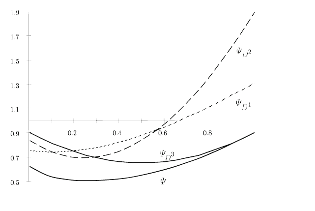
8.5 Generalized Bounds 371

for

= 0.1 . Note how the convex hull of the graphs of the approximationsappears

to have similar subgradients to that of

. This observation appears to hold quite

generally, as indicated by the computational tests in Birge and Wets [1989].

Fig. 5 Graphs of

(solid line) and the approximations,

(dashed lines).

The separable bounds in

can also be enhanced by, for example, including ﬁxed

values (due to known entries in h ) in the right-hand sides of (5.18). Other pos-

sibilities are to combine the component approximations on an interval instead of

assuming that they may apply for all positive multiples of the v

. In this case, the

solution for some interval of v

multiples can serve as a constraint for determin-

ing solutions for the next v

i+1

. This procedure is carried out in Birge and Wallace

[1988]. It appears especially useful for problems with bounded random variables

and networks (Wallace [1987]).

To improve on these bounds and obtain some form of convergence requires re-

laxation of complete separability. For example, pairs of random variables can be

considered together. In this way, more precise bounds can be found. Determination

of these terms is, however, problem-speciﬁc. In general, the structure of the prob-

lem must be used to obtain the most efﬁcient improvements on the basic separable

approximation bounds.

So far, we have presented bounds for the recourse function with a ﬁxed

value.

In the next subsection, we consider how to combine these approximations into so-

lution algorithms where x varies from iteration to iteration. In the case of the sepa-

rable bounds, this implementation results from a dualization that turns the difﬁcult

convex hull operation into a simpler supremum operation.

372 8 Evaluating and Approximating Expectations

c. General-moment bounds

Many other bounds are possible in addition to those presented so far. A general

form for many of these bounds is found through the solution of an abstract linear

program, called a generalized moment problem. This problem provides the lowest

or highest expected probabilities or objective values that are possible given certain

distribution information that can be written as generalized moments. In this sub-

section, we present this basic framework, some results using second moments, and

generalizations to nonlinear functions. Concepts from measure theory appear again

in this development.

To obtain bounds that hold for all distributions with certain properties, we can

ﬁnd P ∈ P , a set of probability measures on (

) , to extremize a moment

problem. We let B

be the Borel ﬁeld of ℜ

where ℜ

⊃

. We use probability

measures deﬁned directly on B

to simplify the following discussion. We wish to

ﬁnd:

P ∈P a set of probability measures on (

)

s. t.



(

)P(d

) ≤

, i = 1,...,s ,



(

)P(d

, i = s + 1,...,M ,

to maximize



)P(d

) , (5.27)

where M is ﬁnite and the v

are bounded, continuous functions. A solution of

(5.27) obtains an upper bound on the expectation of g with respect to any proba-

bility measure satisfying the conditions given earlier. We could equally well have

posed this to ﬁnd a lower bound.

Problem (5.27)isageneralized moment problem (Krein and Nudel’man [1977]).

When the v

are powers of ξ , the constraints restrict the moments of

with re-

spect to P . In this context, (5.27) determines an upper bound when only limited

moment information on a distribution is available.

Problem (5.27) can also be interpreted as an abstract linear program, i.e., a lin-

ear program deﬁned over an abstract space, because the objective and constraints are

linear functions of the probability measure. The solution is then an extreme point

in the inﬁnite-dimensional space of probability measures. The following theorem,

proven in Karr [1983, Theorem 2.1], gives the explicit solution properties. We state

it without proof because our main interests here are in the results and not the partic-

ular form of these solutions. Readers with statistics backgrounds may compare the

result with the Neyman-Pearson lemma and the proof of the optimality conditions

as in Dantzig and Wald [1951]. For details on the weak

∗

topology that appears in

the theorem, we refer the reader to Royden [1968].

8.5 Generalized Bounds 373

Theorem 7. Suppose

is compact. Then the set of feasible measures in (5.27),

P , is convex and compact (with respect to the weak

∗

topology), and P is the

closure of the convex hull of the extreme points of P . If g is continuous relative to

, then an optimum (maximum or minimum) of



g(x,ξ)P(dξ) is attained at an

extreme point of P . The extremal measures of P are those measures that have

ﬁnite support, {

,...,

}, with L ≤M + 1 , such that the vectors

⎛

⎜

⎝

(

)

(

)

(

)

⎞

⎟

⎠

, ...,

⎛

⎜

⎝

(

)

(

)

(

)

⎞

⎟

⎠

(5.28)

are linearly independent.

Kemperman [1968] showed that the supremum is attained under more general

continuity assumptions and provides conditions for P to be nonempty. Dupaˇcov´a

(formerly

Z´aˇckov´a) [1976, 1977, 1966] pioneered the use of the moment problem as

a bounding procedure for stochastic programs in her work on a minimax approach to

stochastic programming. She showed that (5.27) attains the Edmundson-Madansky

bound (and the Jensen bound if the objective is minimized) when the only constraint

in (5.27)is v

, i.e., the constraints ﬁx the ﬁrst moment of the probability mea-

sure. She also provided some properties of the solution with an additional second-

moment constraint ( v

(x)=

) for a speciﬁc objective function g . Frauendorfer’s

[1988b] results can be viewed as solutions of (5.27) when the constraints satisfy all

of the joint moment conditions.

To solve (5.27) generally, we consider a generalized linear programming proce-

dure.

Generalized Linear Programming Procedure for the Generalized Moment

Problem (GLP)

Step 0. Initialization. Identify a set of L ≤ M + 1 linearly independent vectors as

in (5.28) that satisfy the constraints in (5.27). (Note that a phase one–objective

(Dantzig [1963]) may be used if such a starting solution is not immediately avail-

able. For N = 1 , the Gaussian quadrature points may be used.) Let r = L ,

= 1;

go to 1.

Step 1. Master problem solution. Find p

≥ 0,..., p

≥ 0 such that

∑

l=1

= 1 ,

∑

l=1

(

≤

, l = 1,...,s ,