Chow T.L. Mathematical Methods for Physicists: A Concise Introduction

Подождите немного. Документ загружается.

But if

A is an in®nite matrix, then

A is orthogonal if and only if both (3.31a) and

(3.31b) are simultaneously satis®ed.

Now taking the determinant of both sides of Eq. (3.32), we have (det

A

 1,

or det

A 1. This shows that

A is non-singular, and so

ÿ1

exists.

Premultiplying (3.32) by

ÿ1

we have

ÿ1



: 3:33

This is often used as an alternative way of de®ning an orthogonal matrix.

The elements of an orthogonal matrix are not all independent. To ®nd the

conditions between them, let us ®rst equate the ijth elem ent of both sides of



I; we ®nd that

k1

 

: 3:34a

Similarly, equating the ijth element of both sides of

A 

I, we obtain

k1

 

: 3:34b

Note that either (3.34a) and (3.34b) gives 2nn  1 relations. Thus, for a real

orthogonal matrix of order n, there are only n

ÿ nn  1=2  nn ÿ 1=2 diÿer-

ent elements.

Unitary matrix

A matrix

U u



satisfying the relations



; 3:35a

U 

3:35b

is called a unitary matrix. If

U is a ®nite matrix satisfying both (3.35a) and

(3.35b), then

U must be a square matrix, and we have



U 

I: 3:36

This is the complex generalization of the real orthogonal matrix. The elements of

a unitary matrix may be complex, for example



1 i

i 1



is unitary. From the de®nition (3.35), a real unitary matrix is orthogonal.

Taking the determinant of both sides of (3.36) and noting that

det

det

U)*, we have

det

Udet

U*  1orjdet

Uj1: 3:37

116

MATRIX ALGEBRA

This shows that the determinant of a unitary matrix can be a complex number of

unit magnitude, that is, a number of the form e

i

, where  is a real number. It also

shows that a unitary matrix is non-singular and possesses an inverse.

Premultiplying (3.35a) by

ÿ1

, we get



ÿ1

: 3:38

This is often used as an alternative way of de®ning a unitary matrix.

Just as in the case of an orthogonal matrix that is a special (real) case of a

unitary matrix, the elements of a unitary matrix satisfy the following conditions:

k1

 

;

k1

 

: 3:39

The product of two unitary matrices is unitary. The reason is as follows. If

and

are two unitary matrices, then













I; 3:40

which shows that U

is unitary.

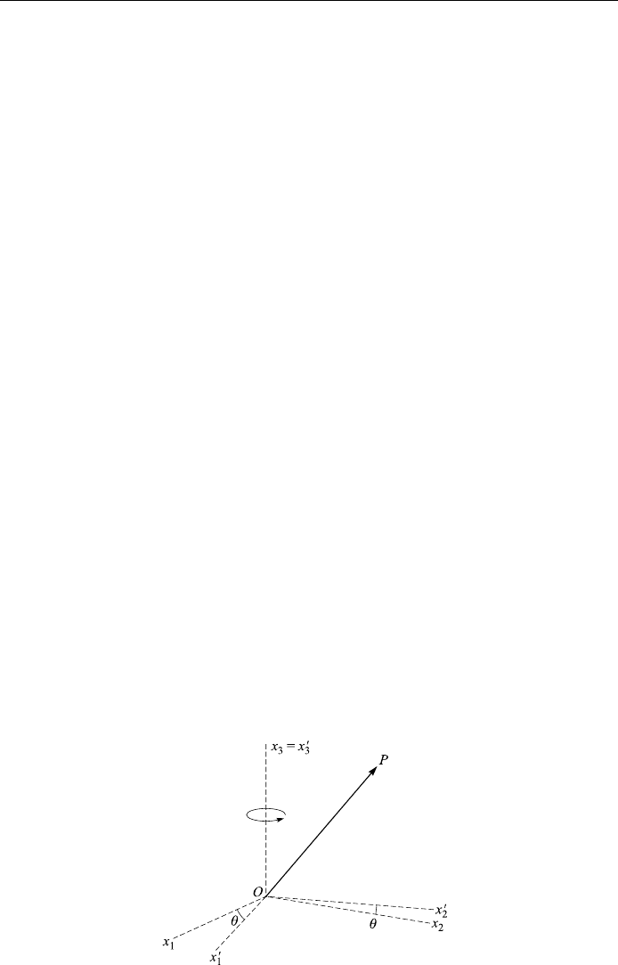
Rotation mat rices

Let us revisit Example 3.5. Our discussion will illustrate the power and usefulness

of matrix methods. We will also see that rotation matrices are orthog onal

matrices. Consider a point P with Cartesian coordinates x

; x

 (see Fig.

3.2). We rotate the coordinate axes about the x

-axis through an angle  and

create a new coordinate system, the primed system. The point P now has the

coordinates x

; x

 in the primed system. Thus the position vector r of

point P can be written as

r 

i1



i1

: 3:41

117

ROTATION MATRICES

Figure 3.2. Coordinate change by rotation.

Taking the dot product of Eq. (3.41) with

and using the orthonormal relation



 

(where 

is the Kronecker delta symbol), we obtain x

 r 

Similarly, we have x

 r 

and x

 r 

. Combining these results we have



j1





j1



; i  1; 2; 3: 3:42

The quantities 





are called the coecients of transformation. They are

the direction cosines of the primed coordinate axes relative to the unprimed ones







 cosx

; x

; i; j  1; 2; 3: 3:42a

Eq. (3.42) can be written conveniently in the following matrix form





3:43a





X; 3:43b

where

and

X are the column matrices,

 is called a transformation (or

rotation) matrix; it acts as a linear operator which transforms the vector X into

the vector X

. Strictl y speaking, we should describe the matrix

 as the matrix

representation of the linear operator

. The concept of linear operator is more

general than that of matrix.

Not all of the nine qua ntities 

are independent; six relations exist among the



, hence only three of them are independent. These six relations are found by

using the fact that the magnitude of the vector must be the same in both systems:

i1

x





i1

: 3:44

With the help of Eq. (3.42), the left hand side of the last equation becomes

i1

j1



ý!

k1



ý!



i1

j1

k1



;

which, by rearranging the summations, can be rewritten as

k1

j1

i1



ý!

This last expression will reduce to the right hand side of Eq. (3.43) if and only if

i1



 

; j; k  1; 2; 3: 3:45

118

MATRIX ALGEBRA

Eq. (3.45) gives six relations among the 

, and is known as the orthogonal

condition.

If the primed coordinates system is generated by a rotation about the x

-axis

through an angle  as shown in Fig. 3.2. Then from Example 3.5, we have

 x

cos   x

sin ; x

ÿx

sin   x

cos ; x

 x

: 3:46

Thus



 cos ; 

 sin ; 

 0;



ÿsin ; 

 cos ; 

 0;



 0;

 1:

We can also obtain these elements from Eq. (3.42a). It is obvious that only three

of them are independent, and it is easy to check that they satisfy the condition

given in Eq. (3.45). Now the rotation matrix takes the simp le form



cos  sin  0

ÿsin  cos  0

001

3:47

and its transpose is





cos  ÿsin  0

sin  cos  0

001

Now take the product







cos  sin  0

ÿsin  cos  0

001

cos  ÿsin  0

sin  cos  0

001



100

010

001



which shows that the rotation matrix is an orthogonal matrix. In fact, rotation

matrices are orthogonal matrices, not limited to

 of Eq. (3.47). The proof of

this is easy. Since coordinate transformations are reversible by interchanging old

and new indices, we must have



ÿ1

ÿ



old



new



new



old

 





ÿ

Hence rotation matrices are orthogonal matrices. It is obvious that the inverse of

an orthogonal matrix is equal to its transpose.

A rotation matrix such as given in Eq. (3.47) is a continuous function of its

argument . So its determinant is also a continuous function of  and, in fact, it is

equal to 1 for any . There are matrices of coo rdinate changes with a determinant

of ÿ1. These correspond to inversion of the coordinate axes about the origin and

119

ROTATION MATRICES

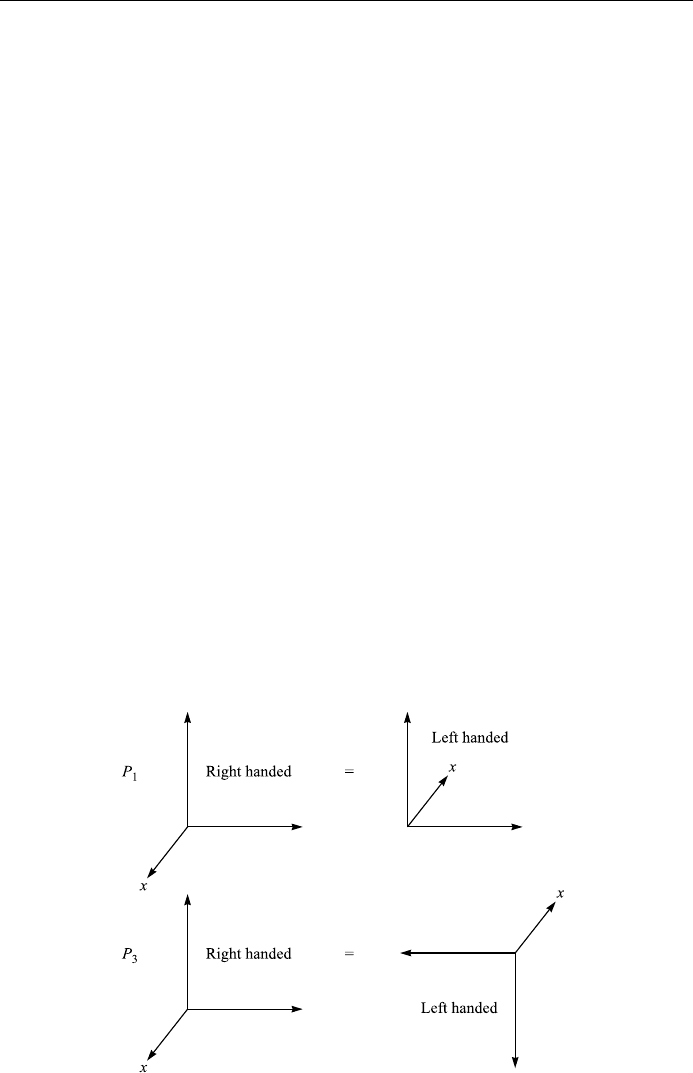
change the handedness of the coordinate system. Example s of such parity trans-

formations are



ÿ100

010

001

;



ÿ100

0 ÿ10

00ÿ1

;

 I:

They change the signs of an odd number of coordinates of a ®xed point r in space

(Fig. 3.3).

What is the advantage of using matrices in describing rotation in space? One of

the advantages is that successive transform ations 1 ; 2; ...; m of the coordinate

axes about the origin are described by successive matrix multiplications as far

as their eÿects on the coordinates of a ®xed point are concerned:

1





2





1

; ...; then

m





mÿ1





mÿ1







X 

where

R 



mÿ1





is the resultant (or net) rotation matrix for the m successive transformations taken

place in the speci®ed manner.

Example 3.9

Consider a rotation of the x

-, x

-axes about the x

-axis by an angle . If this

rotation is followed by a back-rotation of the same angle in the opposite direction,

120

MATRIX ALGEBRA

Figure 3.3. Parity transformations of the coordinate system.

that is, by ÿ, we recover the original coordinate system. Thus

Rÿ

R

100

010

001



ÿ1



R:

Hence

ÿ1



Rÿ

cos  ÿsin  0

sin  cos  0

001



;

which shows that a rotation matrix is an orthogonal matrix.

We would like to make one remark on rotation in space. In the above discus-

sion, we have considered the vector to be ®xed and rotated the coordinate axes.

The rotation matrix can be thought of as an operator that, acting on the unprimed

system, transforms it into the primed system. This view is often called the passive

view of rotation. We could equally well keep the coordinate axes ®xed and rotate

the vector through an equal angle, but in the opposite direction. Then the rotation

matrix would be thought of as an operator acting on the vector, say X, and

changing it into X

. This procedure is called the active view of the rotation.

Trace of a matrix

Recall that the trace of a square matrix

A is de®ned as the sum of all the principal

diagonal elements:

A 

It can be proved that the trace of the product of a ®nite number of matrices is

invariant under any cyclic permutation of the matrices. We leave this as home

work.

Orthogonal and unitary transformations

Eq. (3.42) is a linear transformation and it is called an orthogonal transformation,

because the rotation matrix is an orthogonal matrix. One of the pr operties of an

orthogonal transformation is that it preserves the length of a vector. A more

useful linear transformation in physics is the unitary transformation:

Y 

X 3:48

in which

X and

Y are column matrices (vectors) of order n  1 and

U is a unitary

matrix of order n  n. One of the properties of a unitary transformation is that it

121

TRACE OF A MATRIX

preserves the norm of a vector. To see this, premultiplying Eq. (3.48) by



) and using the condition

U 

I, we obtain

Y 

X 

X 3:49a

k1



k1

: 3:49b

This shows that the norm of a vector remains invariant under a unitary transfor-

mation. If the matrix

U of transformation happens to be real, then

U is also an

orthogonal matrix and the transformation (3.48) is an orthogonal transformation,

and Eqs. (3.49) reduce to

Y 

X; 3:50a

k1



k1

; 3:50b

as we expected.

Similarity transformation

We now consider a diÿerent linear transformation, the similarity transformation

that, we shall see later, is very useful in diagonalization of a matrix. To get the

idea about similarity transformations, we consider vectors r and R in a particular

basis, the coordinate system Ox

, which are connected by a square matrix

R 

Ar: 3:51a

Now rotating the coordinate system about the origin O we obtain a new system

(a new basis). The vectors r and R have not been aÿected by this

rotation. Their components, however, will have diÿerent values in the new system,

and we now have



: 3:51b

The matrix

in the new (primed) system is called similar to the matrix

A in the

old (unprimed) system, since they perform same function. Then what is the rela-

tionship between matrices

A and

? This information is given in the form

of coordinate transformation. We learned in the previous section that the com-

ponents of a vector in the primed and unprimed systems are connected by a

matrix equation similar to Eq. (3.43). Thus we have

r 

and R 

;

122

MATRIX ALGEBRA

where

S is a non-singular matrix, the transition matrix from the new coordinate

system to the old system. W ith these, Eq. (3.51a) becomes



ÿ1

Combining this with Eq. (3.51) gives



ÿ1

S; 3:52

where

and

A are similar matrices. Eq. (3.52) is called a similarity transforma-

tion.

Generalization of this idea to n-dimensional vectors is straightforward. In this

case, we take r and R as two n-dimensional vectors in a particular basis, having

their coordinates connected by the matrix

A (a n  n square matrix) through Eq.

(3.51a). In another basis they are connected by Eq. (3.51b). The relationship

between

A and

is given by Eq. (3.52). The transformation of

A into

ÿ1

is called a similarity transformation.

All identities involving vectors and matrices will remain invariant under a

similarity transformation since this arises only in connection with a change in

basis. That this is so can be seen in the following two simple examples.

Example 3.10

Given the matrix equation

B 

C, and the matrices

C subjected to the

same similarity transformation, show that the matrix equation is invariant.

Solution: Since the three matrices are all subjected to the same similarity trans-

formation, we have



ÿ1

;



ÿ1

;



ÿ1

and it follows that



ÿ1



ÿ1



ÿ1



ÿ1



ÿ1



Example 3.11

Show that the relation

AR 

Br is invariant under a similarity transformation.

Solution: Since matrices

A and

B are subjected to the same similarity transfor-

mation, we have



ÿ1

;



ÿ1

we also have



SR; r



Sr:

123

SIMILARITY TRANSFORMATION

Then



ÿ1

SR

AR and



ÿ1

Sr

thus



We shall see in the following section that similarity transformations are very

useful in diagonalization of a matrix, and that two similar matrices have the same

eigenvalues.

The matrix eigenvalue problem

As we saw in preceding sections, a linear transformation generally carries a vector

X x

; x

; ...; x

 into a vector Y y

; y

; ...; y

: However, there may exist

certain non-zero vectors for which

AX is just X multiplied by a constant 

AX  X: 3:53

That is, the transformation represented by the matrix (operator)

A just multiplies

the vector X by a number . Such a vector is called an eigenvector of the matrix

and  is called an eigenvalue (German: eigenwert) or characteristic value of the

matrix

A. The eigenvector is said to `belong ' (or correspond) to the eigenvalue.

And the set of the eigenvalues of a matrix (an operator) is called its eigenvalue

spectrum.

The problem of ®nding the eigenvalues and eigenvectors of a matrix is called an

eigenvalue problem. We encounter problems of this type in all branches of

physics, classical or quantum. Various methods for the approximate determina-

tion of eigenvalues have been developed, but here we only discuss the

fundamental ideas and concepts that are important for the topics discussed in

this book.

There are two parts to every eigenvalue problem. First, we compute the eigen-

value , given the matrix

A. Then, we compute an eigenvector X for each

previously computed eigenvalue .

Determination of eigenvalues and eigenvectors

We shall now demonstrate that any squ are matrix of order n has at least 1 and at

most n distinct (real or complex ) eigenvalues. To this purpose, let us rewrite the

system of Eq. (3.53) as



A ÿ 

IX  0: 3 :54

This matrix equation really consists of n homogeneous linear equations in the n

unknown elements x

of X:

124

MATRIX ALGEBRA

ÿ x

 a

  a

 0

 a

ÿ x

  a

 0

...

 a

   a

ÿ x

 0

;

3:55

In order to have a non-zero solution, we recall that the determinant of the coe-

cients must be zero; that is,

det

A ÿ 

I

ÿ  a

 a

ÿ   a

 a

ÿ 

 0: 3:56

The expansion of the determinant gives an nth order polynomial equation in ,

and we write this as



 c



nÿ1

 c



nÿ2

  c

nÿ1

  c

 0; 3:57

where the coecients c

are functions of the elements a

A. Eq. (3.56) or (3.57)

is called the characteristic equation corresponding to the matrix

A. We have thus

obtained a very important result: the eigenvalues of a square matrix

A are the

roots of the corresponding charact eristic equation (3.56) or (3.57).

Some of the coecients c

can be readily determined; by an inspect ion of Eq.

(3.56) we ®nd

ÿ1

; c

ÿ1

nÿ1

a

 a

a

; c

 det

A: 3:58

Now let us rewrite the characteristic polynomial in terms of its n roots



;

; ...;



 c



nÿ1

 c



nÿ2

  c

nÿ1

  c

 

ÿ 

ÿ   

ÿ ;

then we see that

ÿ1

nÿ1



 



; c

 





: 3:59

Comparing this with Eq. (3.58), we obtain the following two important results on

the eigenva lues of a matrix:

(1) The sum of the eigenvalues equals the trace (spur) of the matrix:



 



 a

 a

a

 Tr

A: 3:60

(2) The product of the eigenvalues equals the determinant of the matrix:





 det

A: 3:61

125

THE MATRIX EIGENVALUE PROBLEM