Crank J. Free and Moving Boundary Problems

312

Analytical solution

of

seepage problems

Polubarinova-Kochina (1962) gives series expansions of some of the

integrals in

her

solution and presents graphical results for dams of various

dimensions. Cryer

(1976a) evaluated

the

values quoted in Table 7.1. Ozis

(1981) used Cryer's values of

a and

(3

in the first line

of

Table 7.1 and

evaluated the position of the free boundary. His results are given in Table

7.2 normalised to

H = 1, e

=~,

h = i; they were obtained on a

CDC

7600 computer using single-precision arithmetic and a Gauss algorithm

with 64 points to evaluate the integrals.

The

separation point

is

given by

h. = 0.5295. These values agree

to

within one

in

the fourth decimal place

with those quoted by Elliott and Ockendon (1982), who also give

solutions for the other two sets of parameters in Table 7.1.

Polubarinova-Kochina (1962) gave details of the cases of a trapezoidal

dam with and without evaporation

and

of seepage in two media of

different permeabilities. She also introduced a general theory for more

complicated problems in which more than three singular points exist

(Polubarinova-Kochina 1939, Nos. 5, 6).

8.

Numerical solution of

free-boundary problems

8.1.

Numerical solutions

A

NUMBER

of

free-boundary problems were formulated in Chapter 2 and

frequent reference was made

to

this present chapter for more details of

how numerical solutions can

be

obtained. Various numerical methods

have been devised and they fall into two broad classes.

In

the first class

the

techniques are applied to the problem as originally formulated in the

physical plane.

In the second class the problem is recast in a different

form, e.g. by introducing

the

Baiocchi variable

or

some suitable change of

coordinates, and the transformed problem

is solved numerically.

The

choice

of

method is influenced by various factors, apart from the problem

itself, such as the development

of

more powerful numerical techniques for

solving partial differential equations

and

the computing facilities availa-

ble.

It

is

not

really possible to make a well-founded statement that

one

method is in general superior to all

other

methods, though

I:Dore

re-

stricted claims can be made in relation to certain types

of

problem

especially

if

some

one

aspect

of

the solution is of particular interest.

8.2. Trial free-boundary methods

The

simple

dam

problem illustrated in Fig. 2.1 and formulated by

equations (2.7-12)

is taken as

the

model for describing the numerical

techniques. All trial free-boundary methods are variations

on

one

basic

theme.

An

initial estimate

is

made

of

the free boundary

FD

in Fig. 2.1, to

be

denoted for convenience by

reO).

A first approximation

<f>~O)(x,

y)

is

computed

of

the solution

<f>

0

of

the boundary value problem defined in the

seepage region by the appropriate partial differential equation and the

conditions

on

the 'fixed' boundaries together with one of the two condi-

tions

on

the free boundary.

An

improved approximation to the free

boundary,

r(l),

is taken as the line

on

which the remaining free boundary

condition is satisfied according to the first approximate solution,

<f>~.

Thus,

when

an

approximation

r(k)

has been obtained for the problem

of

Fig. 2.1

and

n(k) is

the

corresponding seepage region,

<f>~k)

is computed from (2.7),

314

Numerical solution

of

free-boundary problems

i.e. V

2

<t>(k)

=0,

in

n(k)

satisfying

the

conditions (2.8), (2.10), (2.11), and

the

second

of

(2.9)

on

r(k). Given r(k) and

<t>~k>,

a new trial free boundary,

r(k+l), is found by requiring that

the

first of (2.9) should

be

satisfied

on

r(k+l).

The

iterative process

is

terminated when successive

rs

agree

to

a

specified accuracy.

It

is convenient

to

discuss

the

two parts

of

the

iterative cycle separately

even though, in practice, the solving

of

the elliptic differential equation

on

the

approximated seepage region

n(k)

and the movement

of

the

trial free

boundary from r(k)

to

r(k+l) are interrelated.

8.2.1. Computation

of

approximate trial solutions

The

numerical solution

of

fixed boundary-value problems is a specialist

topic which has been extensively studied. A useful survey is edited by

Gladwell and Wait (1979). A discretized form of a problem can

be

based

on

finite differences

or

finite elements.

In

each case what is ultimately

required is the solution

of

a system

of

algebraic equations, not necessarily

linear, and again there is a choice between direct and iterative methods of

solution. 'Introductory textbooks by Smith (1978)

on

finite-difference

methods and by Davies (1980)

on

finite elements include references

to

more comprehensive accounts

and

Gladwell and Wait (1979) is a valuable

source-book. Cryer

(1976b) included many references in a brief review

of

different methods and

of

the

influence

of

developments in computing-

facilities.

More

details about finite differences and free-boundary prob-

lems are given by Cryer (1970) and Mogel and Street (1974) and about

finite element calculations by Neuman and Witherspoon (1970), Taylor

and Brown (1967), Finn (1967), Larock and Taylor (1976), and

Bathe

and Khoshgoftaar (1979).

Shaw and Southwell (1941) first used finite-difference relaxation

techniques in a trial free-boundary method. Many similar calculations

followed and are described by Southwell (1946), Allen (1954), Bickley

(1964). Digital computation was first attempted by Young

et al. (1955)

and Arms and Gates (1957).

After

a short period of equation solving by

computer with

adju.<;tment

of

the

free boundary by hand, a computer was

virtually always used for

the

whole operation after 1960. Cryer (1976b)

listed a number of

the

early papers

on

trial free-boundary solutions based

on

finite differences.

The

matrix which results when the partial derivatives are replaced by

finite-difference ratios

at

every point of a grid covering

the

seepage

region, for example, is usually sparse and well structured. Iterative

methods, e.g. Gauss-Seidel

or

SOR, which take advantage of the special

matrix features, are described for example by Varga (1962), Young

(1971), and Yanenko (1971),

and

suitable direct methods by Bunch and

Rose (1976), Reid (1971),

and

Buzbee and

Dorr

(1974).

Both

methods

Trial free-boundary methods

315

are discussed by Reid (1979). The relative efficiencies of these methods

when applied to free boundary problems reflect their performance in

fixed boundary problems.

One

or

two special features may also influence

their usefulness, however. Thus, an approximate solution

cf>~k-l)

provides

a better than usual initial approximation to

cf>~k),

since the only change

is

in r, which

is

expected to

be

smalI. H the algebraic equations are

non-linear it

is

likely that an iterative method will be more efficient in a

free boundary context. Care in ordering the equations may improve the

efficiency

of

a direct method since many of the computations needed to

carry out a Gaussian elimination, for example, for

cf>~k>,

will have been

performed

to

find

cf>~k-l).

As

to

the

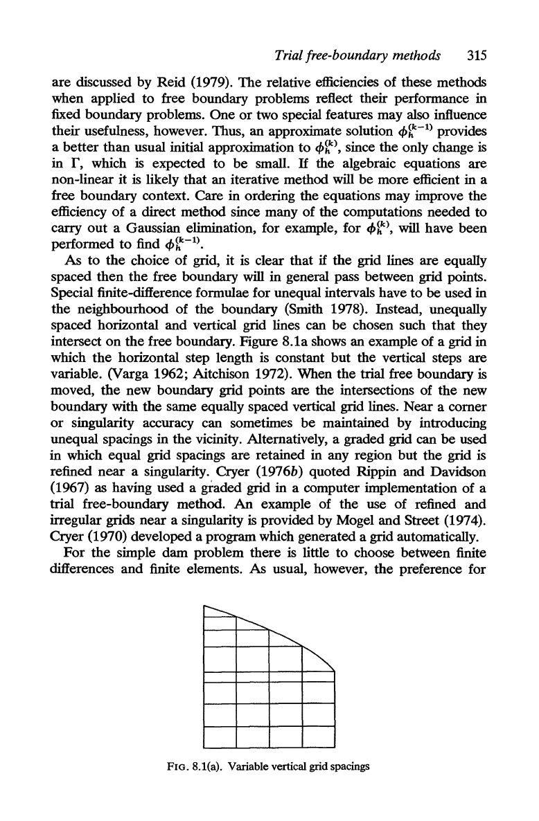
choice of grid, it

is

clear that

if

the grid lines are equally

spaced then

the

free boundary will in general pass between grid points.

Special finite-difference formulae for unequal intervals have to be used in

the neighbourhood of the boundary (Smith 1978). Instead, unequally

spaced horizontal and vertical grid lines can be chosen such that they

intersect on the free boundary. Figure 8.1a shows an example of a grid in

which

the

horizontal step length is constant but the vertical steps are

variable. (Varga 1962; Aitchison 1972). When the trial free boundary

is

moved,

the

new boundary grid points are the intersections of the new

boundary with the same equally spaced vertical grid lines. Near a corner

or singularity accuracy can sometimes be maintained by introducing

unequal spacings in the vicinity. Alternatively, a graded grid can be used

in which equal grid spacings are retained in any region but the grid

is

refined

near

a singularity. Cryer (1976b) quoted Rippin and Davidson

(1967) as having used a graded grid in a computer implementation of a

trial free-boundary method.

An

example of the use of refined and

irregular grids near a singularity

is

provided by Mogel and Street (1974).

Cryer (1970) developed a program which generated a grid automatically.

For

the simple dam problem there

is

little to choose between finite

differences and finite elements. As usual, however, the preference for

L::::::"

...............

~

FIG.8.1(a). Variable vertical grid spacings

316

Numerical solution

of

free-boundary problems

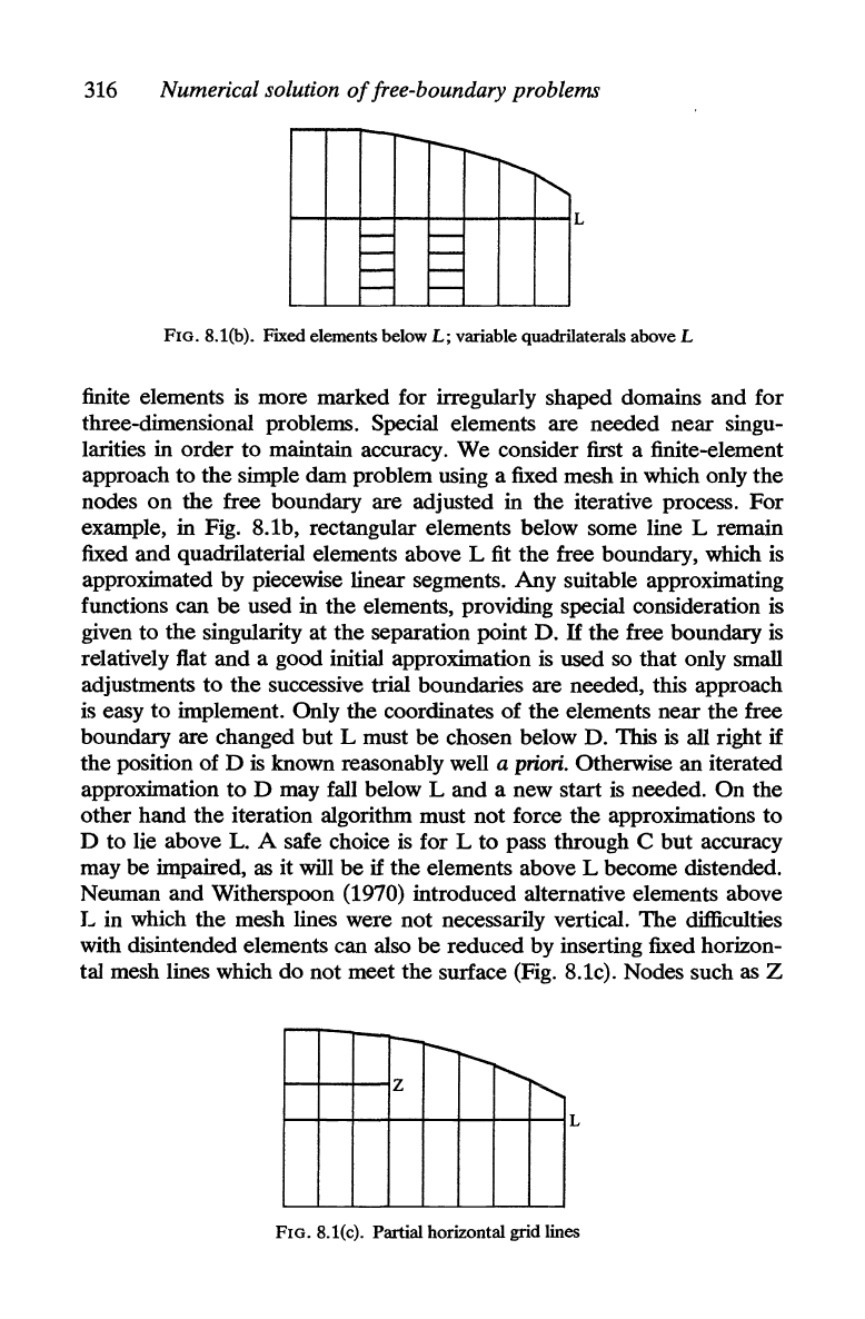
FIG. 8.1(b). Fixed elements below

L;

variable quadrilaterals above L

finite elements is more marked for irregularly shaped domains

and

for

three-dimensional problems. Special elements are

needed

near

singu-

larities in

order

to

maintain accuracy.

We

consider first a finite-element

approach

to

the

simple

dam

problem using a fixed mesh in which only

the

nodes

on

the

free boundary are adjusted in

the

iterative process.

For

example, in Fig. 8.1b, rectangular elements below some line L remain

fixed

and

quadrilaterial elements above L fit

the

free boundary, which is

approximated by piecewise linear segments.

Any

suitable approximating

functions can

be

used in

the

elements, providing special consideration is

given

to

the

singularity

at

the

separation point

D.

If

the

free boundary is

relatively fiat

and

a good initial approximation is used so

that

only small

adjustments

to

the

successive trial boundaries

are

needed, this approach

is easy

to

implement. Only

the

coordinates

of

the

elements

near

the

free

boundary are changed

but

L must

be

chosen below

D.

This

is

all right

if

the

position of D is known reasonably well a

priori.

Otherwise

an

iterated

approximation

to

D may fall below L

and

a new start is needed.

On

the

other

hand

the

iteration algorithm must

not

force

the

approximations

to

D

to

lie above L. A safe choice is for L

to

pass through C

but

accuracy

may

be

impaired, as it will

be

if

the

elements above L become distended.

Neuman

and

Witherspoon (1970) introduced alternative elements above

L in which

the

mesh lines were

not

necessarily vertical.

The

difficulties

with disintended elements can also

be

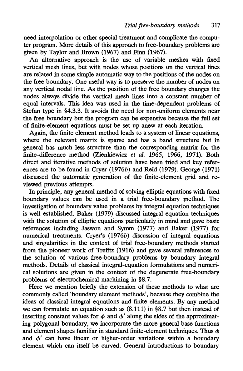
reduced by inserting fixed horizon-

tal mesh lines which

do

not

meet

the

surface (Fig. 8.1c). Nodes such as Z

r--r--

""'"-

z

i"'-...r'"

........

L

FIG. 8.1(c). Partial horizontal grid lines

Trial free-boundary methods

317

need

interpolation

or

other

special treatment

and

complicate

the

compu-

ter

program. More details

of

this approach

to

free-boundary problems are

given

by

Taylor

and

Brown (1967) and Finn (1967).

An

alternative approach is

the

use

of

variable meshes with fixed

vertical mesh lines,

but

with nodes whose positions

on

the

vertical lines

are

some simple automatic way

to

the

positions

of

the

nodes

on

the

free boundary.

One

useful way is

to

preserve

the

number

of

nodes

on

any vertical nodal line.

As

the

position

of

the

free boundary changes

the

nodes always divide

the

vertical mesh lines into a constant

number

of

equal intervals. This idea was used in

the

time-dependent problems

of

Stefan type

in

§4.3.3.

It

avoids

the

need

for non-uniform elements

near

the

free boundary

but

the

program can

be

expensive because

the

full set

of

finite-element equations must

be

set

up

anew

at

each iteration.

Again,

the

finite element method leads

to

a system

of

linear equations,

where

the

relevant matrix is sparse

and

has a

band

structqre

but

in

general has much less structure

than

the

corresponding matrix for

the

finite-difference method (Zienkiewicz et

al.

1965, 1966, 1971).

Both

direct

and

iterative methods

of

solution have

been

tried

and

key refer-

ences are

to

be

found in Cryer (1976b)

and

Reid

(1979). George (1971)

discussed

the

automatic generation

of

the

finite-element grid

and

re-

viewed previous attempts.

In

principle, any general method

of

solving elliptic equations with fixed

boundary values can

be

used in a trial free-boundary method.

The

investigation

of

boundary value problems by integral equation techniques

is well established.

Baker

(1979) discussed integral equation techniques

with

the

solution

of

elliptic equations particularly in mind

and

gave basic

references including Jaswon

and

Symm (1977)

and

Baker

(1977) for

numerical treatments. Cryer's (1976b) discussion

of

integral equations

and

singularities in

the

context

of

trial free-boundary methods started

from

the

pioneer work

of

Trefftz (1916)

and

gave several references

to

the

solution

of

various free-boundary problems by boundary integral

methods. Details

of

classical integral-equation formulations and numeri-

cal solutions are given in

the

context

of

the

degenerate free-boundary

problems

of

electrochemical machining in §S.7.

Here

we mention briefly

the

extension

of

these methods

to

what are

commonly called 'boundary element methods', because they combine

the

ideas

of

classical integral equations

and

finite elements. By any method

we can formulate

an

equation such as (S.111)

in

§S.7

but

then instead

of

inserting constant values for

<p

and

<P'

along

the

sides

of

the

approximat-

ing polygonal boundary, we incorporate

the

more

general base functions

and

element shapes familiar in standard finite-element techniques. Thus

<p

and

<P'

can have linear

or

higher-order variations within a boundary

element which can itself

be

curved. General introductions

to

boundary

318

Numerical solution

of

free-boundary problems

element methods are given by Brebbia (1980 pp. 3-33) and Wrobel

and

Brebbia (1981), and applications to porous flow free-boundary problems

by Brebbia and Chang

(1979), Brebbia and Dominguez (1977), Radoj-

kovic

(1980), Awater (1980), and Bischoff (1980). The last author in-

cludes particularly water movement in non-homogeneous media and

refers to Butterfield

(1978) and

to

Liggett (1977) for an iterative proce-

dure to improve the free-boundary position. Lennon

(1980) solved a

number of free-surface problems in porous media in two and three space

dimensions and with axial symmetry by using boundary elements.

He

includes axisymmetric and three-dimensional solutions in aquifers of

infinite and finite depths, ponds, and wells. Some comparisons with

the

linearized perturbation solutions of Dagan (1967) are made. Approxi-

mate solutions obtained by replacing a well, for example, by an axial line

sink are found to

be

adequate for practical purposes away from the wall

of the well. A multiple-well problem is solved with four wells

at

positions

with respect to coordinates

(x,

y, z) given by

(d,

0, z), (0,

d,

z),

(-d,

0, z),

(0,

-d,

z), where z is vertical, d is constant, and

-2<z<-1.

An

example

takes

d = 1.2,

the

well

at

(d, 0, z)

to

be a pumping well with a rate +0.6'IT,

and the other three are re-charge wells with rates -O.lS'IT, -0.4'IT, and

-O.OS'IT

respectively. Numerous references include Wu (1976) on

the

boundary integral method using various approximation techniques, Lig-

gett and Liu

(1977, 1979) on unsteady flows, and Liu and Liggett (1977,

1978, 1979),

the second paper being on an efficient numerical method for

two-dimensional steady ground-water problems.

In

finite-element methods the dependent variable u is approximated by

where the

cf>i

are piecewise polynomial finite-element basis functions.

If

on the other hand the functions

cP;

are defined over the whole region we

have a global method described by Delves

(1979). Thus in a global

Galerkin method the functions could be chosen to satisfy all

or

some of

the boundary conditions and the coefficients

a; determined by collocation

or least squares, for example. So-called regional methods employ a global

expansion over a few sub-regions in more complicated regions, for

example, for which the construction of sensible global basis functions

is

difficult

or

convergence is slow. Details of implementing global and

regional methods are outlined by Delves

(1979) with examples. Cryer

(1976b) referred

to

global methods

and

quoted an application by Kirk-

ham

(1964) to the problem of axisymmetric porous flow towards a fully

penetrating well. Also Mason and Farkas

(1972) considered a freshwater

canal

in

the centre of a long island with an impervious surface.

Trial free-boundary methods

319

Cryer (1976b) also mentioned several graphical

and

analogue

methods, including the Hele-Shaw analogue discussed in §2.12.1.

8.2.2. Moving the

free

boundary

Once

the

approximate solution

</>~k)

of the elliptic equation has been

obtained for

an

estimated ,position

r(k)

of

the

free boundary there

remains

the

problem of moving the free boundary

to

an improved

approximation position,

r(k+1),

such that the remaining free-boundary

condition is satisfied.

Of

course, this means in general

that

the

first

condition is no longer satisfied and further iteration is

needed__

There

appears

to

be

no general rule for deciding which boundary condition

should

be

used in solving

the

elliptic equation and which for moving

the

free boundary.

The

choice depends

on

the

problem and sometimes one is

clearly

more

convenient

or

efficient than

the

other.

In

porous flow problems where the condition

</>

= y is

to

be satisfied on

the free boundary,

an

improved position,

r(k+l),

of

the

boundary can

simply

be

taken

as the line

on

which

</>

=

y,

found by interpolation

on

the

approximate solution,

</>(k),

of the boundary-value problem. Thus Aitchi-

son (1972), for example, moved

the

boundary points along

the

vertical

grid lines.

To

find

the

new value of

Yj'

the

intercept of the free boundary

with the

jth

vertical grid line, j = 0, 1,

...

,

n,

the

values

of

</>~k)

- Y along

the

jth

grid line are examined.

The

zero

of

</>~k)

- Y

is

found by linear

interpolation

and

taken as

the

value of

Yj.

Cryer (1976b) classified methods

of

moving the boundary

as

local,

integral,

or

global.

(i)

Local methods.

In

a local method adjustments

to

r(k)

are made at

individual points

on

the basis

of

the

error,

C</>(k>,

where

the

second

boundary condition

is written

C(

</»

=

O.

Thus

if

ap~k)

is

computed at m

points

11

k

),

l~j~m,

and

if

ap~k)fO

at

11

k

),

then the point

11

k

)

is moved

to

I1k+l)

where

the

boundary condition is better satisfied in some sense.

In

general,

the

displacement is programmed by conditions

CA..(h

k

) at

p,k+l)

= 0

p(k+l)

-

p(k)

=

a(k)

d(k)

(8.1)

'I'

J , J J J

I'

where dJk) is a specified unit vector

and

aJk) is a parameter. Various ways

of choosing

both

d

and

a have been tried (Cryer, 1976b).

Possible choices for

dJk)

are (a) the outward normal

to

r(k)

at

11

k

);

(b)

the

unit vector in one

of

the coordinate directions;

(c)

the outward

conormal

to

r(k)

at

11

k

),

e.g.

if

the elliptic equation is

~

(fl

a</»+~

(f2

a</»

= 0

ax ax

ay ay

and

the

outward normal is n =

(n!>

n~,

the

unit outward conormal is

the

320

Numerical solution

of

free-boundary problems

vector

{(flnl)2+

(f2n2)2)!

with

the

possible advantage

that

the

boundary conditions

are

often

expressed in

tenns

of

the

conormal;

or

(d) some arbitrarily specified

dfk).

A Newton-type interpretation of

afk)

can

be

used by defining

f}k)(a) =

Gp(k)CI1k)

+

ad}k»)

(8.2)

and

computing

or

estimating (df/da)",=o so

that

a~k)

=

-fk)(O)/

{~f}k)(a)}

. (8.3)

da

«=0

Alternatively,

if

G/>(P) is

of

the

form Gp(P)=F{</>(p),

</>n(P),

P}=O, a}k)

has been defined

by

(8.4)

i.e.

the

dependence of

</>(k)

on

P is neglected between

Pfk)

and

p}k+1).

If

the

free-boundary condition C for porous flow problems is written

C =

</>

- y =

0,

where

</>

is

velocity potential, (8.4) with

dfk)

chosen in

the

direction

of

the

y-axis leads

to

Pfk+l)

=

(xf+\

y~k+1»),

where

X}k+l)

=

X}k)

and

y}k+l) =

</>~k)(~k»).

Neumann

and

Witherspoon (1970) used this

idea

and

also incorporated certain refinements. Similarly for porous problems

Taylor (1966)

and

Kealy

and

Williams (1971) wrote C as p = 0, with p

being pressure

and

then

p}k+1)_

p~k)

=

(3p~k)CI1k»)djk>,

(8.5)

where

the

factor

(3

and

djk)

are

arbitrarily chosen. A similar

but

more

general .choice is ajk) =

G{c<p(~k»)},

where G is

an

arbitrary function;

(8.5) corresponds

to

G(C)

= (3c.

For

C</>(p)

written in

the

Dirichlet form

C</>(p)

=

</>(P)

+

'Yl(P)

= 0,

(8.3) becomes

0:

{</>(k)(p)

+

'Yl

(P)}P=I1k)

The

quantity

O'Yl/oa

is readily computed

and

if

the

first free-boundary

condition is written o</>/oa+'Y2=0, o</>(k)/oa=-'Y2. Otherwise

o</>(k)/oa

must

be

estimated, probably numerically. Cryer (1976b) quoted several

authors who

have

used this method.

He

also

quoted

a

number

of

Trial free-boundary methods

321

instances in which the Neuman form,

C(P)

=

n

(P)

+

'Y2(P)

= 0, was used

as

the

second free-boundary condition, and concluded that for both

Dirichlet and Neuman conditions local methods of moving the boundary

have been used very successfully.

Doha

(1977) compared numerically various finite-difference methods

of iterating the position of the free boundary.

He

considered that the effect

of

the

change in

the

domain

on

the solution should

be

taken into account

by using the total derivative

of

in computing

C<f>(k).

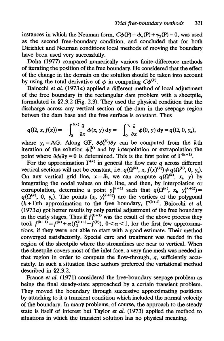
Baiocchi

et

al. (1973a) applied a different method of local adjustment

of

the free boundary in

the

rectangular dam problem with a sheetpile,

formulated in §2.3.2 (Fig. 2.3). They used the physical condition

that

the

discharge across any vertical section

of

the dam in the seepage region

betwen

the

dam

base and the free surface is constant. Thus

I

f(X)

a

lY'

a

q(O,

x, f(x)) = - -

(x, y)

dy

= - -

<1>(0,

y)

dy

=q(O,

0,

Ys),

o

ax

0

ax

where

y.

=

AG.

Along GF,

a<l>~k)/ay

can

be

computed from the

kth

iteration

of

the

solution

~k)

and by interpolation

or

extrapolation the

point where

a<l>lay

= °

is

determined. This is the fitst point

of

r(k+l).

For

the approximation

r(k)

in general the flow

rate

q across different

vertical sections

will not

be

constant, i.e. q(O(k),

x,

f(X)(k»)

=/=

q(O(k), 0,

y,,).

On

any vertical grid line, x =

ih,

we can compute q(O(k),

Xi,

y) by

integrating the nodal values

on

this line, and then, by interpolation

or

extrapolation, determine a point

y~k+l)

such that

q(O(k>,

Xi,

y~k+l»)

=

q(O(k),

0,

Ys).

The

points

(Xi,

y~k+l»)

are the vertices

of

the polygonal

(k+1)th

approximation to the free boundary,

r(k+l).

Baiocchi

et

al.

(1973a) got better results by only partial adjustment of the free boundary

in the early stages. Thus

if

f~k+l)

was

the

result

of

the above process they

took

tk+l)=tk)+a(f~k+l)_tk»),

O<a<l,

for

the

first.

few approxima-

tions,

if

they were not able to start with a good estimate. Their method

converged satisfactorily. Special care and treatment was needed in the

region

of

the sheetpile where the streamlines are near to vertical. When

the sheetpile covers most of the inlet face, a very fine mesh was needed in

that region in order to compute the flow-through,

q, sufficiently accu-

rately.

In

such a situation these authors preferred the variational method

described in §2.3.2.

France

et

aI.

(1971) considered the free-boundary seepage problem as

being the final steady-state approached by a certain transient problem.

They moved the boundary through successive approximating positions

by attaching to

it

a transient condition which included the normal velocity

of

the boundary.

In

many problems, of course, the approach to the steady

state is itself

of

interest but Taylor et al. (1973) applied the method to

situations in which

the

transient solution has no physical meaning.

Crank J. Free and Moving Boundary Problems

Подождите немного. Документ загружается.