Crank J. Free and Moving Boundary Problems
Подождите немного. Документ загружается.

332
Numerical solution
of
free-boundary problems
known exactly. Furthermore, by defining
f(c)={(1+c
2
)}!-.j1O,
we find
that
C(k+l)
= C(k)-f(C(k»)/f(c(k»), which
is
the Newton iterative formula for
the
solution of f(c) = 0 from the initial guess
c(o)..
Since f(c)
is
convex for
c~o
and
f(O)
<0
it follows that for any initial guess c(O)<O the sequence
of the trials
r(k)
converges quadratically
to
the
true free boundary. Thus
the simple problem lends support
to
Garabedian's claim (1956) that his
rewriting of
the
boundary conditions leads
to
quadratic convergence and
points
to
the
connection with Newton's method. Cryer (1968) found that
numerical
result~
for a more complicated problem in stellar evolution
behaved like those for the model problem which was chosen
to
resemble
it.
8.3. Boundary singularities
Singularities commonly occur
on
a fixed boundary in boundary-value
problems. They may be associated with sudden changes in the direction of
the boundary, as
at
a re-entrant corner,
or
with mixed boundary condi-
tions. Much attention has been paid
to
these singularities and methods
include mesh refinement for both finite differences and finite elements,
and
the
use of modified finite-difference approximations
or
singular finite
elements in which the local analytical form of
the
singularity is somehow
incorporated. Various other techniques are based
on
integral equations,
power series, dual series, Fourier series, and removal of
the
singularity.
Conformal transformation methods have proved particularly efficient and
highly accurate for
the
solution
of
elliptic problems.
Good
summaries
together with
other
basic references are given by Fox (1979) for finite
differences, by Wait (1979) for finite elements, Delves (1979) for global
and regional methods, and by Scheffler and Whiteman (1979) for
conformal-mapping techniques. Many other references
to
these and other
methods are quoted by Furzeland
(1977b).
In
addition
to
such generally occurring singularities, free-boundary
problems often have a singularity
at
the separation point where
the
free
boundary meets a fixed boundary, as, for example,
at
point D in Fig. 2.1
for the simple dam problem.
Aitchi~on
(1972) used complex variable
methods
to
determine
the
shape of
the
free boundary near the separation
point and incorporated the local analytical solution into a finite-difference
scheme in order to improve its accuracy.
Starting with
the
dam problem defined by equations (2.7-11) in Chap-
ter
2, but taking
Yl
= 1,
Y2
= d, and
Xl
= L in Fig. 2.1, Aitchison (1972)
moved the origin of
the
(x,
y) coordinates
to
D and added a constant
to
c(J
so that
cfJo
=
O.
In terms of the stream function
"',
the condition
ac(Jlan
= 0
on
DF
becomes '" = 0,
and
the problem is
to
determine the complex variable
Boundary singularities
333
N 'I'
x-o
D x D
,z;-o
x='l'
N
M
z-plane
w-plane
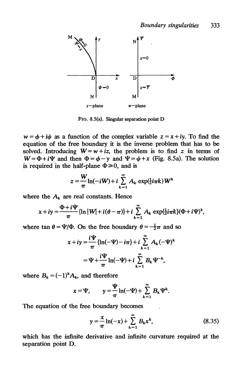
FIG. 8.5(a). Singular separation point D
w =
</>
+
it{!
a<;
a function
of
the
complex variable z = x + iy.
To
find the
equation
of
the free boundary it
is
the inverse problem that has
to
be
solved. Introducing W = w + iz,
the
problem
is
to
find z in tenns of
W=<I>+i'Yand
then
<I>=</>-y
and '1'=
t{!+x
(Fig. 8.5a).
The
solution
is required in
the
half-plane
<1>;;;,,0,
and
is
z = W In(
-iW)
+ i f
Ak
exp@i1Tk)
W
k
1T
k=l
where
the
Ak
are real constants. Hence
x +
iy
=
<1>+
i'Y
{In
IWI
+
i(6
-1T)}+
i f
~
exp{!i1Tk}(<I>
+ i'Y)k,
1T
k=l
where
tan
6 =
'1'/<1>.
On
the
free boundary 6 =
-~1T
and
so
x+iy=i'Y
{In(-'Y)-i1T}+i
f
Ak(-'Yl
1T
k=l
where
Bk = (-l)kAk> and therefore
x ='1',
'1'
00
y=-ln(-'Y)+
L Bk'Yk.
1T
k=l
The
equation of
the
free boundary becomes
(8.35)
which has
the
infinite derivative and infinite curvature required
at
the
separation point
D.

334
Numerical solution
of
free-boundary problems
Aitchison (1972) described two ways of incorporating the analytical
expression (8.35) for the free boundary and the corresponding solution
for the potential
</>
into a finite-difference solution. A trial free-boundary
method was described in §8.2.2 in which the zero of
</>
- Y along any
vertical grid line is found by linear interpolation along the line
and
taken
to
be
the new intersection of
the
free boundary with that ordinate. This
method cannot be used
to
find
the
value
Yno
the ordinate of the separation
point
D,
because
</>
= Y along
the
whole of
CD
in Fig. 2.1. Instead,
Yn
ha~
to be found by fitting a suitable curve through
Yn-l>
Yn-2'
••••
Such a
curve is given by equation (8.35).
The
position of the origin of coordi-
nates for (8.35)
is
not known and so the curve based
on
r terms of the
infinite sum can
be
fitted through r + 1 of the points
Yi'
conveniently taken
as
Yn-r-l>
Yn-r>""
Yn-l say. Aitchison (1972) quoted numerical results
for the free-boundary curve for
r having values 0, 1, and 2 and concluded
that
r = 1 gave satisfactory results for most applications. Grid sizes chosen
for
the
finite-difference calculations were 1/24, 1/36, and 1/48.
An
alternative procedure included use of values of
</>
from the analyti-
cal solution at grid points in
the
neighbourhood of the singularity.
In
this
case, only one term of the infinite sum was taken, so that
z =
(W/'IT)ln(
-iW)
+ A
W,
(8.36)
where W
= w + iz.
The
value
of
A is determined during
the
calculation of
Yn
and can
be
taken
as
known.
In
order
to
find
</>
at a grid point P(x, y) a
form of Newtonian iteration was used based on
the
function
f(w),
where
f(W)
=
(W/'IT)ln(-iW)
+ A W -
Zp,
(8.37)
wher~
Zp
i~
a known constant for a selected point P.
The
iterative cycle
needed
to
find
the
root of
f(W)
= 0 is defined by
f(~)
=
(WJ'IT)ln(-i~)+
A~
-
Zp,
f(~)
= In(
-i~)
+ 1 +
A,
'IT
~+1
=
~
-
f(~)/f(~).
A good enough starting value is provided by the values calculated for the
previous free-boundary position.
The
value of W yielded by the Newton
iteration satisfies (8.37) with
Z =
Zp,
and w = W -
iz
and hence
</>p
follow
immediately.
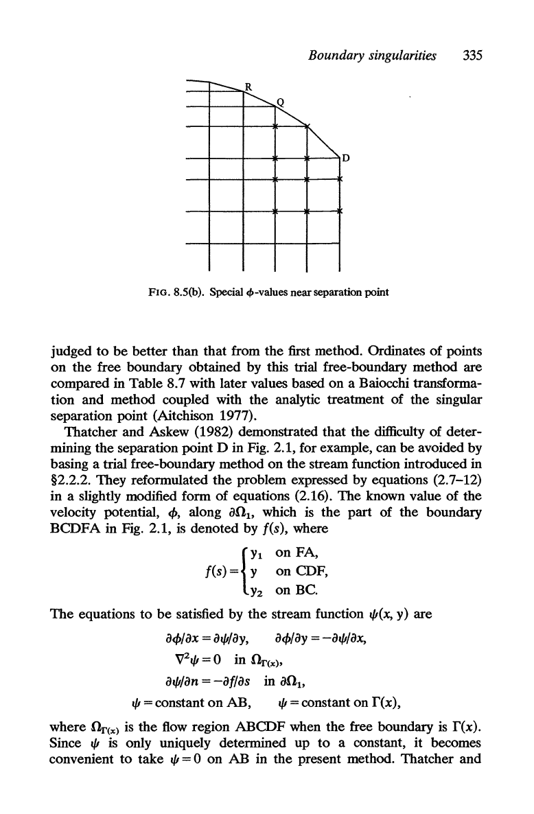
Aitchison (1972) used
</>
values determined in this way
at
the
grid
points marked by crosses shown in Fig. 8.5b, and
the
curve Y =
(X/'IT)ln(-x)+
Ax
was fitted through the points
Rand
Q
to
give values of
Yn-l>
Yno
and
A.
For a particular grid size the value of
Yn
obtained by
using
the
second method, which included the analytical values of
</>,
was
Boundary singularities
335
--...........,
R
~Q
.~
~
D
FIG.
S.5(b). Special q,-values near separation point
judged
to
be
better
than
that
from
the
first method. Ordinates
of
points
on
the
free boundary
obtained
by
this trial free-boundary
method
are
compared
in
Table
8.7 with
later
values based
on
a Baiocchi transforma-
tion
and
method
coupled with
the
analytic
treatment
of
the
singular
separation
point (Aitchison 1977).
Thatcher
and
Askew (1982) demonstrated
that
the
difficulty of
deter-
mining
the
separation
point
D in Fig. 2.1, for example,
can
be
avoided by
basing a trial free-boundary
method
on
the
stream function introduced in
§2.2.2.
They
reformulated
the
problem
expressed
by
equations (2.7-12)
in
a slightly modified
form
of
equations (2.16).
The
known value
of
the
velocity potential,
q"
along
001>
which is
the
part
of
the
boundary
BCDFA
in Fig. 2.1, is
denoted
by
f(s), where
{
Yl
on
FA,
f(s) = Y
on
CDF,
Y2
on
Be.
The
equations
to
be
satisfied
by
the
stream
function IjI(x, y)
are
aq,/ax
=
aljl/Oy,
aq,/ay
=
-aljl/ax,
VZIjI
= 0 in
fir(x),
aljl/an
=
-of/as
in
001>
IjI
= constant
on
AB,
IjI
= constant
on
f(x),
where
fir(x)
is
the
flow region
ABCDF
when
the
free boundary
is
f(x).
Since
IjI
is only uniquely
determined
up
to
a constant, it becomes
convenient
to
take
IjI
= 0
on
AB
in
the
present method.
Thatcher
and
336
Numerical solution
of
free-boundary problems
A'>kew
(1982) seek the pair
{I/I,
r(x)}
such that
1/1
minimizes
the
functional
I(v)
=
lex)
IVvl
2
d!l+2
fan,
(aflas)v ds,
over trial functions v that are zero along
AB
with
r(x)
chosen so
that
1/1
is
constant there.
The
trial free-boundary method becomes:
(i)
choose
ro
and set
the
iteration index p
=0,
(ii) triangulate
firp
and choose a linear trial function
vp
which satisfies
the condition
vp
= 0
on
AB,
(iii) find
I/I
p
that
minimizes
the
functional
I(
v),
(iv)
find r
p
+
1
by interpolating
or
extrapolating along
the
vertical mesh
lines, such that
on
the
new free-boundary nodes
I/I
p
is
constant and
equal
to
I/I
p
at F.
(v)
set p = p + 1 and go
to
(ii)
if
the procedure has not converged
sufficiently.
The
flow
region
firp
is triangulated by constructing vertical lines,
parallel to
the
y-axis, and having
an
equal number
of
equally spaced
nodes along each vertical line, including the sections
of
the
dam
faces,
AF
and BCD.
One
of
the
nodes is at C.
The
jth
nodes along neighbouring
vertical lines
are
connected and each
of
the resulting quadrilaterals is
triangulated by a diagonal as usual.
The
constant value
of
the
exact solution
1/1
along the free boundary is
the
di'>Charge
q
per
unit length through
the
dam and
the
constant value
evaluated by
the
trial free-boundary method was found by Thatcher and
Askew
to
approach the
true
value
a'>
the convergence criterion was made
smaller. Their ordinates
of
the
free boundary for the simple
dam
agreed
better with those
of
Aitchison (1972) than with Aitchison (1977) except
at the separation point. Re'>ults are also quoted for
the
same
dam
but
with
Y2
= 0, for a vertical-stratified
dam
studied by Oden and Kikuchi
(1980), and for a rotationally-symmetric dam
of
interest in porous-well
problems (Cryer and
Fetter
1979).
8.4. Methods using variable interchange
Various authors have sought
to
avoid some of
the
difficulties associated
with trial free-boundary methods by interchanging
the
dependent variable
with
one
or
more
of
the independent variable'>, e.g. in porous
flow
problems
the
flow
potential is interchanged with
one
of
the
space vari-
ables
x,
y,
which becomes
the
new, dependent variable
to
be
computed.
Finn and Varoglu (1977) proposed a variational formulation
of
porous
flow
through a trapezoidal dam which incorporated a variable domain
of
integration.
In
order
to
generate a finite-element mesh which automati-
cally adjusted
to
the
different trial positions of
the
free boundary, they
Methods using variable interchange
337
specified the nodes by chosen, fixed values of
~
and
y.
The values of x
both within
the
seepage region and on the free boundary, computed on
this fixed, finite-element mesh are
the
solutions of variational equations.
Crank and Ozis
(1980) transformed their problem by the same inter-
change of
variable.<;
and solved a transformed equation in a new fixed
domain in which
the
free boundary became a known straight-line bound-
ary. Again one of
the
space variables was computed in the transformed
domain and simultaneously on the free boundary in a single iterative
process. A wen-established procedure in two-dimensional fluid-flow
problems is
to
interchange both the potential function
~
and the stream
function
1/1_
with
the
two space variables
'x
and
y.
The problem
is
reformulated in
the
~,
rjJ
plane and x, y values are computed in what
is
often a fixed, rectangular region. This 'inverse' approach has been ex-
plored extensively in relation
to
free-boundary problems culminating in a
three-dimensional application described by Jeppson
(1972) in a paper
which gives references
to
earlier work. These different uses of variable
interchange are now
de.<;cribed
in more detail.
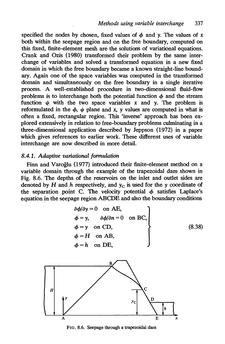
8.4.1. Adaptive variational formulation
Finn and VarogIu
(1977) introduced their finite-element method on a
variable domain through the example of the trapezoidal dam shown in
Fig. 8.6.
The
depths of
the
reservoirs on the inlet and outlet sides are
denoted by
H and h respectively, and
Yc
is
used for
the
y coordinate of
the
separation point C.
The
velocity potential
~
satisfies Laplace's
equation in the seepage region
ABCDE
and also
the
boundary conditions
H
a~/ay
= 0
on
AE,
~=y,
a~/an=O
on BC,
~=y
on
CD,
~=H
on AB,
~=h
on
DE,
FIG. 8.6. Seepage through a trapezoidal
dam
(8.38)
x

338
Numerical solution
of
free-boundary problems
which have
the
same physical significance
as
in the problems formulated
in Chapter 2.
Finn and VarogIu (1977) considered the functional I defined by
1=
J
J{(o<p/oX)2+(o<p/OY)~
dx dy,
(8.39)
o
where the domain n
is
the
seepage region, and both
<p(x,
y) and n may
vary.
The
variation
of
the domain n is constrained by the fact that
the
separation point C can only move along
the
outlet face
CEo
Only
the
free
boundary
BC
and
the
seepage face
CD
can
be
varied;
the
rest
of
the
boundary
of
n is fixed.
Courant and Hilbert (1953) showed that the first variation
of
I when
the domain
of
integration can
be
varied takes
the
form
81=-2
JJ
VZ
<p
8
<p
dx
dy+2
J
(o<p
ax
+
o<p
Oy)
8<p
ds
oX
on
oyon
o
ABCDE
where
8<p
denotes the variation
at
a fixed point (x, y) and so
&P
=
8<P
-
o<p
8x
-
o<p
8y.
oX
oy
(8.41)
The
line integrals in (8.40) are taken round
the
boundary
of
n,
indicated
by
ABCDE;
n is the outward normal and s is measured along
the
boundary. Admissible functions
<p(x,
y) must satisfy
the
boundary condi-
tions
on
CD, AB,
DE
given in (8.38).
The
admis.',ible variations
of
the
domain n
are
8x
=
8y
= 0
on
AB
and
DE,
8y = 0
on
AB, and so (8.40)
reduces after a slight rearrangement
of
terms to
+2
f
o<p
&P
ds+2
i
o<p
&p
ds
AB
on
GB
on
+ L
e~r(8X
dy-8y
dx). (8.42)
If
8U is defined by
8U=81+
Le
e~)\8xdY-8YdX),
(8.43)
Methods
using
variable interchange
339
the function
cf>(x,
y) which satisfies
the
boundary conditions
on
CD, AB,
DE
in (8.38) and for which
au
defined in (8.43) is zero for all admissible
variations
ax, ay,
&t>
can also
be
shown to satisfy
V2cf>
= 0 in 0 and
acf>/an
= 0 on BC and AB. Thus
the
variational formulation is equivalent
to
the
boundary-value problem with conditions (8.38).
In
order to set
up
a finite-element mesh for the discretization of the
variational problem Finn and Varoglu specify the nodes by chosen fixed
values of
cf>
and
y.
Thus, at a typical node
i,
cf>
and y take arbitrary fixed
values
cf>i(h
:s;;,cf>i
:s;;,H)
and
Yi(O:s;;,Yi
:s;;,c/>;),
except at the separation point C
. (Fig. 8.6) at which
cf>e=
Ye
is
an unknown value
to
be
determined. The
x-coordinates of the nodes
on
the
boundary segments AB,
DE,
and
CD
are known.
The
x-coordinate.'i on the free surface are unknown except for
Xc
which is related
to
Ye
through
the
equation of the exit face of the dam.
Thus
the
problem
is
to
determine the x-coordinates
of
the nodes inside
the
flow
region 0 and on the impermeable base
AB
and the free surface
BC, excluding the end points; the unknown associated with the node
at
the separation point C is taken
to
be
Ye,
making, say, n + 1 unknowns in
alI.
The
di'icretized form of (8.43) can now be written
au
= a L
I;jk
+ L af
ij
(8.44)
ilk
ij
where
The
first summation in (8.44) is carried out over all
the
area elements in
the seepage region
0,
and the second over
all
the line elements on the
free surface BC;
the
direction from i
to
j is the direction from B
to
C
along
the
free surface.
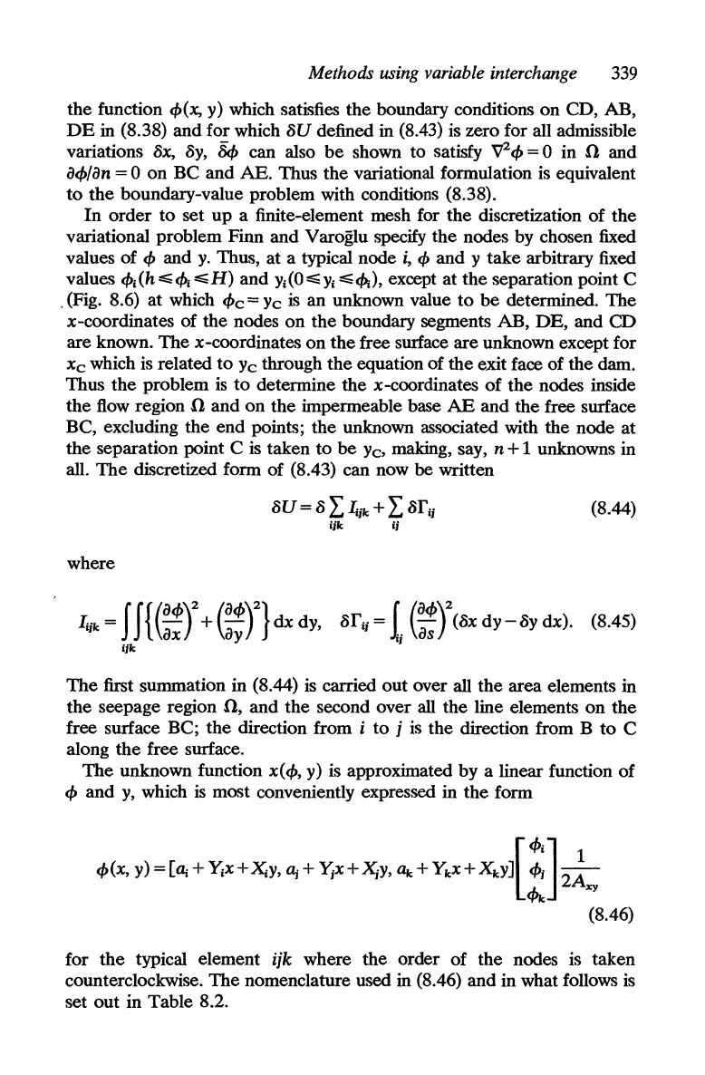
The
unknown function
x(cf>,
y) is approximated by a linear function of
cf>
and y, which
is
most conveniently expressed in the form
for the typical element
ijk
where the order of the nodes is taken
counterclockwise. The nomenclature used in (8.46) and in what follows
is
set out in Table 8.2.

340
Numerical solution
of
free-boundary problems
TABLE
S.2
Definition
of
symbols
for
a typical area element
with vertices
i(Xj,
Yi),
j(Xj,
Yj),
k(x,.;,
Yk)
taken
counterclockwise and
<l>i
=
<I>(Xj,
Y;),
<l>j
=
<I>(Xj,
Yj),
<I>k
=
<I>(Xk,
Yk)
Indices
Symbols
j
k
a
XjYk
-XkYj
XkYi-liYk liYj-XjYi
X
Xk-Xj
li-Xk
Xj-li
Y
Yj-Yk
Yk-Yi
Yi-Yj
<11
<f>Jc
-q,j
q,i-<f>Jc
q,j-q,1
2A,.y
li~
+XjYj+XkYk
2A.,..
c/JtX;
+
q,;Xj
+
cf>rcXrc
2A.,.y
4>.~
+q,jYj+<f>JcYk
Since
a<l>lax
= A.t,yIA"y
and
a<l>lay
= A.t,JA"y
and
<I>
= Y
on
BC,
equa-
tions (S.45)
become
!;jk
=
(A~
+
A~y)1
Axy,
8r
ij
=
(ax~~:~:y)2{!
ay(8Xj
+8Xj)-!
ax(8YI +8Yj)}, (S.47)
by using
the
trapezoidal integration
and
inserting
(a<l>las);'
=
(ayf/(ax
2
+ ay2), m =
i,
j,
where
for
the
element
ij
on
BC,
ay
=
Yj
-
Yi,
ax
=
Xj
-
Xj.
The
discretized
form
of
8U
can
be
written
in
terms
of
variations
of
the
discrete unknowns
Yc
and
x".,
1:,.;;
m
:,.;;
n,
as
n
8U
= L
(tm
8x". +
tn+l
8yc),
m=l
where
the
coefficients
tm
and
tn+l
are
given
by
since
a
tm
=-a
L
!;jk+qm,
m
=1,
2,
...
,
n,
x".
ijk
a
tn+l
=-a
L
!;jk
+qn+b
Yc
ijk
81 = f
(~L
!;ik) 8x". +
(~
L !;ik)
8yc
m=l
ax".
ijk
ayc
ijk
and
Lij
8rij
may
be
written as
n
L
8r
ii
= L
qm
8x". +
qn+l
8yc'
ij
m=l
(S.4S)
(S.49a)
(S.49b)
(S.50a)
(S.50b)
Methods using variable interchange
341
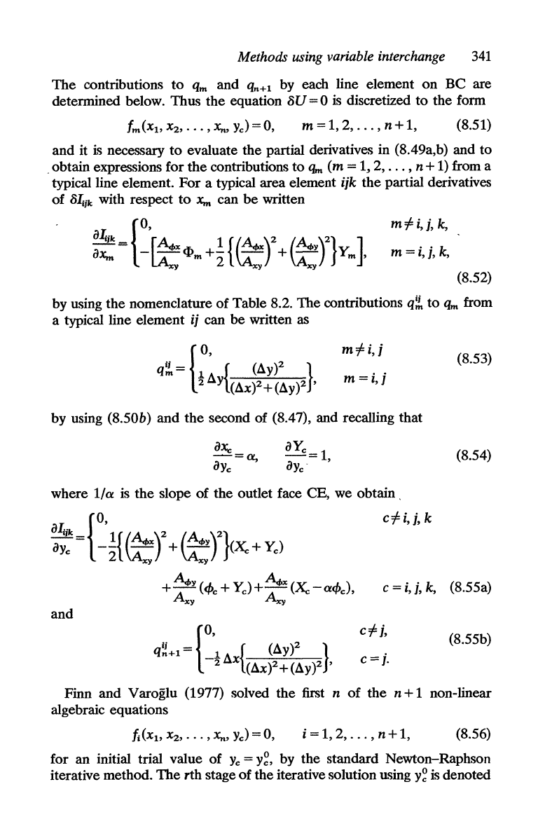
The
contributions
to
qm
and
qn+1
by
each line element on Be are
determined below. Thus
the
equation
5U
= °
is
discretized
to
the form
m=I,2,
...
,
n+l,
(S.51)
and
it
i
..
necessary
to
evaluate the partial derivatives in (S.49a,b) and
to
_ obtain expressions for
the
contributions
to
qm
(m =
1,2,
...
,
n+
1)
from a
typical line element.
For
a typical area element ijk
the
partial derivatives
of
5I;jk
with respect
to
x". can
be
written
m:fi,j,
k,
m
=i,j,
k,
(S.52)
by using
the
nomenclature of Table S.2. The contributions
q!!.
to
qm
from
a typical line element
ij can
be
written as
{
O'
q!!.= 1 { (Ay)2 }
2
Ay
(Ax)2+(Ay)2
'
m:f
i,
j
(S.53)
m=i,j
by using (S.50b) and
the
second of (S.47), and recalling that
(S.54)
where
Ita
is
the
slope of the outlet face CE, we obtain,
c:fi,j,k
c =
i,
j,
k,
(S.55a)
and
c:f
j,
(S.55b)
c=j.
Finn and Varoglu (1977) solved the first n of the n + 1 non-linear
algebraic equations
i = 1, 2,
...
, n + 1,
(S.56)
for an initial trial value of
Yc
=
y~,
by the standard Newton-Raphson
iterative method.
The
rth stage
of
the iterative solution using
y~
is
denoted