Crank J. Free and Moving Boundary Problems
Подождите немного. Документ загружается.

322
Numerical solution
of
free-boundary problems
They started from
the
general equation for seepage
flow
or
irrotational
hydrodynamic flow
~
(lex
aeb)+~
(Icy
aeb)
+~
(k
z
aeb)+Q+C
aeb
=0,
ax ax
ay ay
az
az
at
(S.6a)
where
the
ks are permeabilities, for example, Q is a specified in-flow
and c expresses
the
specific capacity of
the
medium for fluid.
The
usual
fixed boundary conditions are
eb
=
cf>t,(x,
y,
z,
t)
(S.6b)
on
the
part r
1
of the whole boundary
r,
and
on
the
part r
2
where t
x
,
t
y
,
t
z
are the direction cosines of
the
outward normal
on
the
boundary of
the
relevant domain.
In
free-boundary conditions
both
types
of condition have
to
be
satisfied simultaneously
on
the 'free'
part
of
the
boundary.
If
a steady state has
not
been
reached
an
appropriate form of
moving boundary condition is
aeb
aeb aeb
txlex
- +
tyky
- + tzk
z
- =
qo
+
Vns
f
=
qn
ax
ay
az
(S.6d)
say, where
Vn
is
the
normal velocity of
the
boundary
at
any instant,
qo
allows for precipitation
or
other
supply of fluid
to
the
boundary,
and
Sf in
the absence of capillarity is
the
volumetric porosity.
If
the coordinates of
points
on
the free surface are denoted by
Xt,
Yf,
Zf,
all functions of time,
then
Vn
=
txXf+ tyYf+
tzz
f
,
where it= dxf/dt, etc.
Taylor
et al. (1973) proceed with
the
usual finite-element discretization
with
1=1
where usually
the
ebl
are
the
nodal values of
eb
and
Ni
are appropriate
shape functions defined piecewise element by element. Conditions (S.6b)
on
r
1
are automatically satisfied. Discretization
of
(S.6a,b) based
on
a
Galerkin, weighted-residual formulation requires
1
N-[~
(lex
aeba)+~
(ky
a
eb
a
)
o J
ax
ax
ay
ay
a
(k
aeba)
Q a
eb
a
]
(""\
+-
- +
+c-
du=O
az
z
az
at
'
j =
1,2,
...
, m, m < n,
Trial free-boundary methods
323
which becomes after the usual manipulation
H<f,+c
d<f,
+F=O,
(S.7a)
dt
where
~i
= Ie
hji>
j =
1,2,
...
,m, with e denoting a particular finite
element,
h'1
= - r
(a~
lex
aN;
+
a~
ky
aN;+
a~
k
z
aN;)
dO,
J J
o
<
ax ax
ay ay
az
az
<ii
= L
eji>
eji
= [
~eN;
dO, j = 1, 2,
...
,
m,
e
-0-
Fj
= L
Fj,
j = 1, 2,
...
,
m,
e
Fj
= - r
(a~
lex
aN;
+
..
.
)cPl
dO+
jN;.qn
ell' + r
~Q
dO,
J
o
<
ax ax
Joe
in which the first
term
of
Fj
is
only included when
cPi
=
cf>t,.
In
unconfined
seepage problems and irrotational htdrodynamic flow c = 0 and (S.7a)
becomes
H<f,+F=O.
(S.7b)
In
transient free-surface problems there
is
a portion r 3 of the boundary
r where
at
an initial time
cP
is
prescribed but
the
boundary
is
moving
according to
the
condition (S.6d) which must
be
additionally satisfied.
In
such cases Taylor et al. (1973) continue by solving the quasi-static
problem defined by (S.7b)
at
an initial time with
cP
prescribed
on
the
part
of
the boundary r 3 assumed
to
have a known initial position. Then
at
the
nodes
on
the free boundary, r
3,
~
values are calculated, where
and the condition
on
r
3,
F;
=~+
r
N;qn
elI'=0,
.Jr,
(S.7c)
allows the unknown
qn
to
be
computed and hence Vn follows from (S.6d),
i.e.
qn
=
qo
+ Vns
f
as follows.
Let the free-boundary nodes
be
constrained to move along prescribed
lines, e.g. along the vertical coordinate lines z so that
Zf
= z(t).
If
Zf
= I
N;Zi
then the component of
if
in the direction of
Vn
is
{zif
=
{z
IN;ii
and using (S.7c) and qn=qO+ Vns
f
we have
(S.7d)
324
Numerical solution
of
free-boundary problems
On writing
e
iij
==
f
N;s~
dI',
t
(8.7a) gives a system of equations
i
f
=-L-
1
(R-Ro),
and
finally
an
improved free-boundary position follows by moving each
boundary
node
by
aZ
f
=
if
at.
The
transient computation proceeds step
by step
at
till
the
steady state is achieved which
is
the
solution
of
the
appropriate elliptic problem with
oq,/ot
=
O.
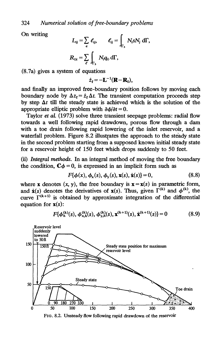
Taylor et al. (1973) solve three transient seepage problems: radial flow
towards a well following rapid drawdown, porous flow through a
dam
with a
toe
drain following rapid lowering
of
the
inlet reservoir,
and
a
waterfall problem. Figure
8.2
illustrates
the
approach
to
the
steady
state
in
the
second problem starting from a supposed known initial steady
state
for a reservoir height
of
150 feet which drops suddenly
to
50
feet.
(ii) Integral methods.
In
an
integral
method
of
moving
the
free boundary
the
condition,
Cq,
= 0, is expressed in
an
implicit form such
as
F{q,(x),
<Px(s),
c/Jy(s),
xes), xes)} = 0,
(8.8)
where x denotes (x, y),
the
free boundary is
x=x(s)
in parametric form,
and
xes) denotes
the
derivatives
of
xes). Thus, given
r(k)
and
q,(k),
the
curve
r(k+l)
is obtained by approximate integration
of
the
differential
equation for xes):
F{q,~k)(S),
q,~~(s),
q,~~~(s),
X(k+l)(S),
X(k+l)(S)}
= 0 (8.9)
100
Steady state
o
150
200
250
300
350
400
FIG. 8.2. Unsteady flow following rapid drawdown
of
the
reservoir
Trial free-boundary methods
325
where
<b~k)(S),
etc., denote approximations at the point
X(k+l)(S),
obtained
by interpolation
if
the
point lies inside the seepage region and by
extrapolation
if
it is outside. Applications
of'
the method' often take
<b(k)(S)
to
be
the value of
<b(k)
at the grid point nearest to
X(k+l)(S).
Cryer
(1976b) reported a number of uses of this method. In the simple dam
problem, for example, an approximation to the velocity field, say
V~k),
can
be determined by differentiating the approximation to the velocity poten-
tial,
<b~k).
The free boundary
is
a streamline for the condition
C<b
=
<bn
= 0
and so an improved approximation,
r(k+l>,
can be obtained by integrating
the velocity field
V(k).
Cryer (1976b) concluded from the practical evidence available that trial
free-boundary methods as described so far are stable and converge
satisfactorily for porous
flow
problems. Any local method can
be
used
and smoothing
is
not required. Where there has been a suspicion of
instability (Taylor and Brown 1967; Neuman and Witherspoon 1970;
Kealy and Busch 1971) it seems to have occurred in the region where the
free boundary joins the seepage surface. The trouble may be associated
with the precise nature of the boundary conditions there, which can
include the
type of singularity discussed by Aitchison (1972) and in §8.3.
Shaw and Southwell (1941) asserted that in porous
flow
problems,
if
the
initial guess
r(O)
for the free boundary
is
horizontal then successive
trials
r(k)
converge monotonely downwards. They based a proof on the
maximum principle.
Cryer
(1976b), however, gives examples of instabilities in more general
free-boundary problems for which global methods may be preferred.
(iii) Global methods. In a global method the solution
is
computed for a
number of independent choices of
r(k)
and then, in principle, it
is
possible
to use inverse interpolation
or
some other technique to determine the
new trial boundary
r(k+l).
For example, the least-squares error in the
boundary condition on
r(k+l)
can be minimized on the evidence of the
dependence of this error on the parameters defining the set of chosen
r(k).
Even so, Fox and Sankar (1973) advise against local improvement of
mesh points by solving an inverse interpolation problem to find a new
position of just one mesh point on
r(k+l),
leaving all other points
untreated.
In
order to avoid the oscillations of the mesh points on
r(k+l)
which local improvement can produce, they propose that all mesh points
should be improved simultaneously. Their algorithm involves solving the
appropriate fixed boundary problem for
n + 1 different choices of r
initially but then only one new fixed-boundary problem has to be solved
per
iteration. Both the problem and the algorithm devised by Fox and
Sankar (1973) have features of general interest and are now described in
more detail.
326
Numerical solution
of
free-boundary problems
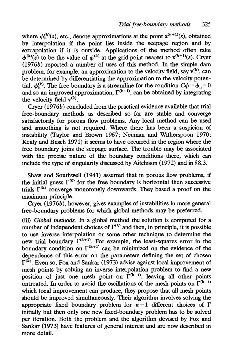
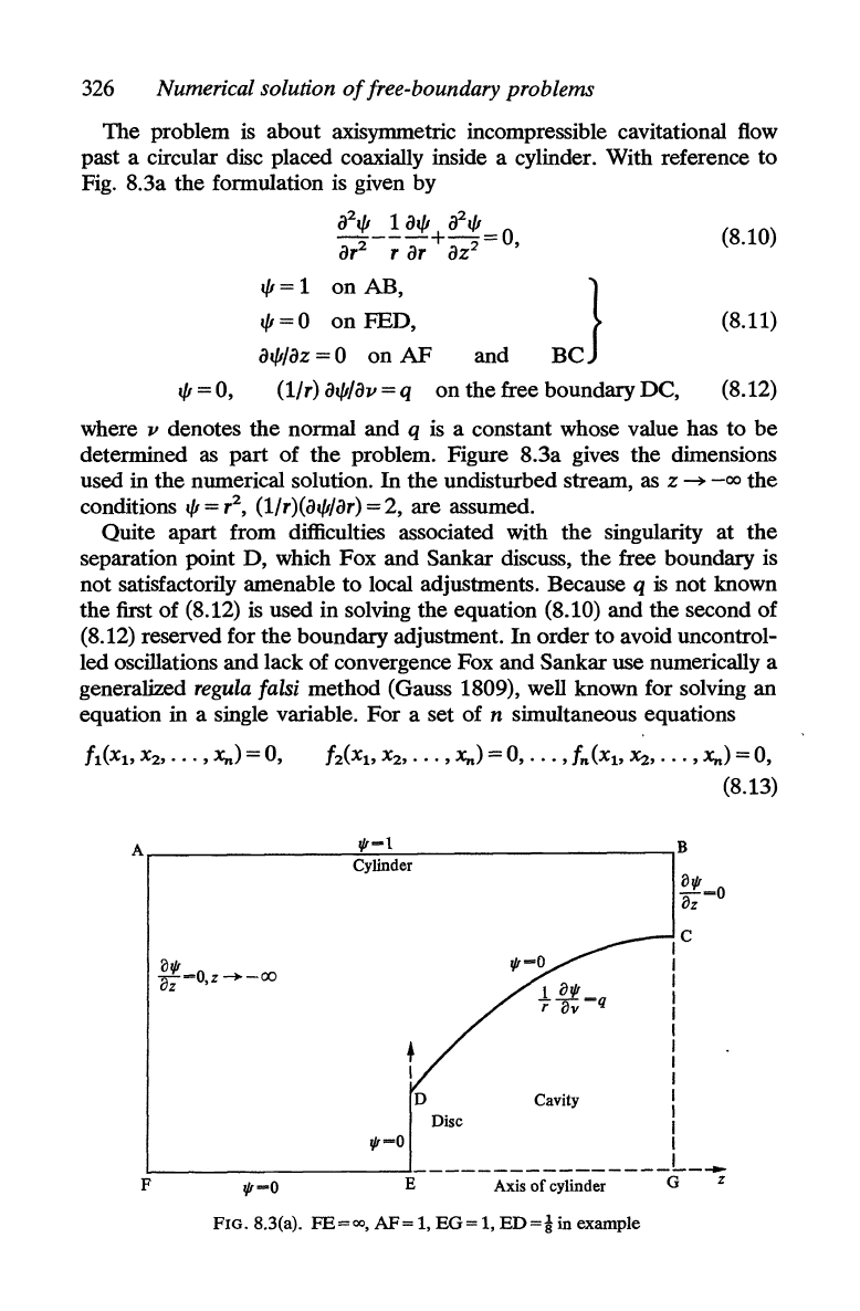
The problem
is
about axisymmetric incompressible cavitational
flow
past a circular disc placed coaxially inside a cylinder. With reference to
Fig. S.3a the formulation is given by
ill/J
1
al/J
a
2
1/J
ar2
--;:
ar
+ az2=0, (S.10)
l/J=1
onAB,
BJ
l/J=O
on FED,
(S.l1)
aWaz=o
onAF
and
l/J
= 0,
(1/r)
al/Jlav
= q
on the free boundary DC,
(S.12)
where v denotes the normal and q
is
a constant whose value has to
be
determined
as
part
of the problem. Figure S.3a gives the dimensions
used in the numerical solution. In the undisturbed stream,
as
z
~
-00
the
conditions
l/J=r2,
(1/r)(al/J/ar)
=2,
are assumed.
Quite apart from difficulties associated with the singularity
at
the
separation point D, which Fox and Sankar discuss,
the
free boundary is
not satisfactorily amenable to local adjustments. Because q
is
not known
the first of (S.12)
is
used in solving the equation (S.10) and the second of
(S.12) reserved for the boundary adjustment. In order
to
avoid uncontrol-
led oscillations and lack of convergence Fox and Sankar use numerically a
generalized
regula falsi method (Gauss lS09), well known for solving an
equation in a single variable. For a set of
n simultaneous equations
f2(Xl>
X2,
..•
, x,.) = 0,
...
,
fn
(Xl>
Xz,
...
, x,.) = 0,
(S.13)
A.-
____________
~~~-~l------------------__.B
Cylinder
D
Cavity
Disc
(:)~-O
(:)z
I
C
I
I
I
I
I
I
I
I
I
I
I
~~
I
L..-
__________________
-:'
________________
L
___
E Axis of cylinder G Z
F
~=O
FIG.8.3(a).
FE
=
00,
AF=
1,
EG=
1,
ED=k
in example
Trial free-boundary methods
327
it
is assumed
that
all the
t,
j = 1, 2,
...
,n,
can
be
computed
at
n + 1
'points' P
=
(x~>'
x~>'
...
,x~»,
i =
1,2,
...
, n +
1.
In
the one-dimensional
solution of
f(x)
= 0,
the
value of x is determined
at
which
the
straight line
ax+b=f
(fortherequiredx,f=O)
(S.14)
joining
the
points
(Xl>
f(Xl» and
(X2,
f(~),
intersects
the
x-axis.
The
relationships
aX
l
+ b =
f(x
l
) ,
lead
to
the
determinantal equation
a~+b=f(~)
(S.lS)
(S.16)
for
x.
In
place
of
(S.14)
and
(S.15), Fox and Sankar take the n equations
allxl
+a12~2.~"
.+b
l
=
O}
a..1Xl
+
a..2
X
2+'
..
+
b,.
= 0
and
the
n
(n
+ 1) equations
allx~)+a12X~)+"
.+b
l
=fl(Pi)}
(i)+
(0+
+b
-f
(P)
~lXl
a2
2
x
2
...
2-
2 i
;=1
2
+1
• "
...
, n
a..1X~)+a..2X~)+",
+b
n
= fn(P
i
)
(S.17)
(S.lS)
respectively
and
solve (S.lS)
to
give an 'improved' point
P=
(Xl>
X2,
...
,x,,). Typical rows
of
n determinantal equations correspond-
ing
to
(S.16) become
fl
(P;) ,
fiP;)""'fn(p;)I:O}
fl
(P;),
fiP;),
...
,
fn
(Pi)\-
0 . 1 2 1
1=
, ,
•.•
,n+
iI(P;), f2(Pi),
...
,fn(P;)1 = 0 (S.19)
The
solution
of
(S.19) is
j = 1, 2,
...
,
n,
(S.20)
where
the
numerator
and
denominator are determinants of which
the
ith
row is shown in each case and i goes from 1
to
n +
1.
The
equations
(S.20) give
the
improved approximate solutions of equations (S.13).
One
of
the
previous Pi is replaced by this new P and the process repeated till
satisfactory convergence is reached.
328
Numerical solution
of
free-boundary problems
r---------------------------------------~B
L-
__________________
~--J---J-----------~---~
E G z
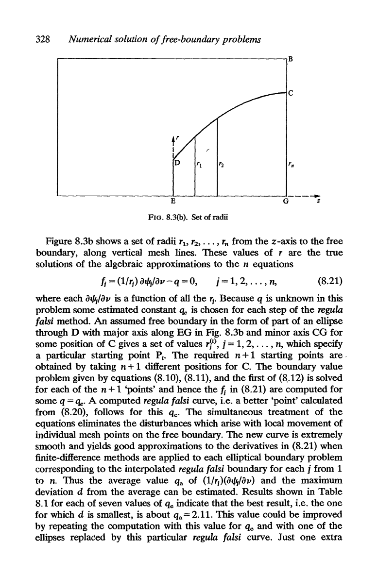
FIG.8.3(b).
Set
of
radii
Figure 8.3b shows a set
of
radii
r1>
r2,
...
,
rn
from
the
z-axis to the free
boundary, along vertical mesh lines. These values of r
are
the
true
solutions
of
the
algebraic approximations
to
the
n equations
j=
1, 2,
...
,
n,
(8.21)
where each
iJt/Ij/iJv
is a function
of
all the
lj.
Because q is unknown in this
problem some estimated constant
qe
is chosen for each step of
the
regula
falsi method.
An
assumed free boundary in
the
form of
part
of an ellipse
through D with major axis along
EG
in Fig. 8.3b and minor axis
CG
for
some position
of
C
give~
a set
of
value~
rJo,
j = 1, 2,
...
,
n,
which specify
a particular starting point
Pi'
The
required n + 1 starting points
are·
obtained by taking n + 1 different positions for C.
The
boundary value
problem given
by
equations (8.10), (8.11), and
the
first
of
(8,.12) is solved
for each
of
the n + 1 'points' and hence the t in (8.21)
are
computed for
some
q =
qe'
A computed
regula
falsi curve, i.e. a
better
'point' calculated
from (8.20), follows for this
qe'
The
simultaneous treatment
of
the
equations e1iminates
the
disturbances which arise with local movement of
individual mesh points
on
the
free boundary.
The
new curve
is
extremely
smooth and yields good approximations
to
the derivatives in (8.21) when
finite-difference methods
are
applied to each elliptical boundary problem
corresponding
to
the
interpolated
regula
falsi boundary for each j from 1
to
n.
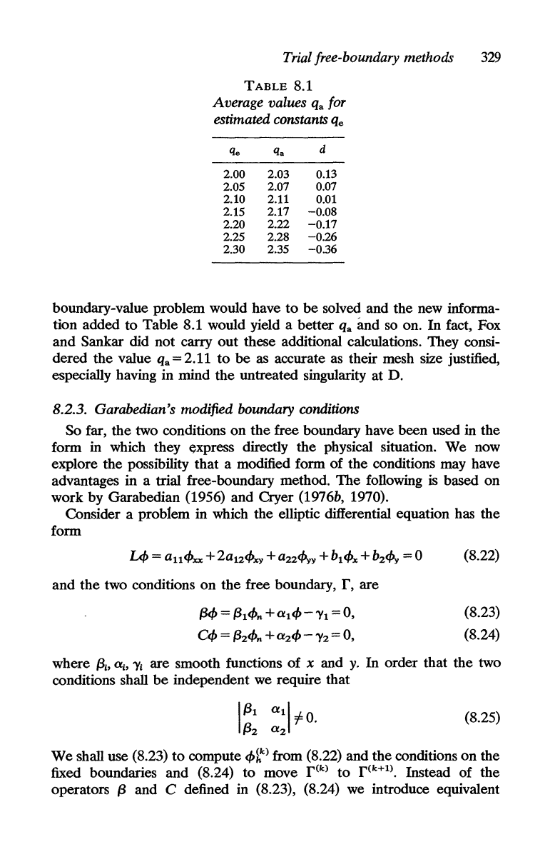
Thus the average value qa of (l/rj)(iJt/ljliJv) and
the
maximum
deviation d from
the
average can
be
estimated. Results shown in Table
8.1 for each
of
seven values of
qe
indicate that
the
best result, i.e. the
one
for which d
is
smallest,
is
about qa = 2.11. This value could
be
improved
by repeating the computation with this value for
qe
and with
one
of
the
el1ipses
replaCed by this particular
regula
falsi curve. Just
one
extra
Trial free-boundary methods
329
TABLE
8.1
Average values qa for
estimated constants
qe
qe qa
d
2.00 2.03 0.13
2.05
2.07 0.07
2.10 2.11
0.01
2.15 2.17
-0.08
2.20
2.22
-0.17
2.25 2.28
-0.26
2.30 2.35
-0.36
boundary-value problem would have
to
be
solved and the new informa-
tion added
to
Table 8.1 would yield a better qa and so on.
In
fact, Fox
and Sankar did not carry
out
these additional calculations. They consi-
dered the value
qa = 2.11
to
be as accurate as their mesh size justified,
especially having in mind the untreated singularity at D.
8.2.3. Garabedian's modified boundary conditions
So far,
the
two conditions on
the
free boundary have been used in the
form in which they express directly the physical situation. We now
explore the possibility that a modified form of the conditions may have
advantages in a trial free-boundary method.
The
following is based on
work by Garabedian (1956) and Cryer
(1976b, 1970).
Consider a problem in which the elliptic differential equation has the
form
and
the
two conditions
on
the free boundary, r, are
(3<1>
=
(31
<bn
+
a1
<I>
-
'V1
= 0,
C<I>
=
(32<bn
+
a2<1>
-
'V2
= 0,
(8.22)
(8.23)
(8.24)
where
(3;.
a;,
'Vi
are smooth functions of x and
y.
In order that the two
conditions shall
be
independent we require that
1
(31
a11::f.O.
(32
a2
(8.25)
We
shall use (8.23)
to
compute
<l>h
k
)
from (8.22) and the conditions
on
the
fixed boundaries and (8.24)
to
move
r(k)
to
r(k+1).
Instead of the
operators
(3
and C defined in (8.23), (8.24)
we
introduce equivalent
330
Numerical solution
of
free-boundary problems
operators
~,
C,
where
~=e11(3+e12C
on
r
=
(3
on
the fixed boundary,
C=
e2l(3 +
e22
C
on
r,
(8.26)
(8.27)
and the
es are smooth functions satisfying a determinantal condition like
(8.25).
The
aim is to choose
~,
C so as to improve convergence
of
a trial
free-boundary method.
When
r(k)
on
which (8.23)
i~
sati~fied
by
q,~k)
is
moved
to
r(k+1)
so
that
(8.24) is satisfied, in general (8.23)
will no longer
be
satisfied. Garabe-
dian's idea was
to
construct
~
so
that
~q,
i~
insensitive
to
movements of
r, i.e.
~
is
stationary with respect
to
normal displacements
of
r,
so
that
(~)n
= 0
on
r. (8.28)
The
coefficients
e;j
can
be
chosen such
that
~
=
(q,n
-
I'll)
+
T(q,
-
I'd
= 0,
Cq,
=
q,-I'12
= 0,
where
T
is
an
arbitrary function, and hence
(~)n
=
q",n
- (I'll)n +
T{
q",
- ("lz)n}
because of (8.30). Thus (8.28) holds
if
(8.29)
(8.30)
T -q",n +
("ll)n
(8.31)
I'll-(I'dn
since (8.29), (8.30) imply
q",
=
I'll.
If
the unit tangent
to
r
is
denoted by
t,
s
is
the distance along r, and K its curvature, we have
on
r
q,t
=
q,.
= (I'lz).
(8.32)
and
as
special cases
of
the Frenet formulae
q,tl
-
Kq,n
=
q,
••
=
(I'd
..
,
q",t
+
K</Jr
= q",. =
(I'll)
•.
(8.33)
The
elliptic equation (8.22) can
be
written as
a~lq",n
+
2a~2<bnt
+
a~2<btt
+
b~
q",
+
b~q,t
= 0,
(8.34)
where the coefficients
a;j
and
b;
are
linear combinations
of
ll;j and
bi.
The
function T can now
be
expressed in terms of
the
I'ij
and their derivatives
and
ll;j,
bi>
K.
An
important special case occurs when (8.22)
is
Laplace's equation and
1'11>
1'22
are constants. Then (8.34) becomes
q",n
+
<btt
= 0 and T = K.
In
practice, the curvature K is not known since r is unknown,
but
T can
be
replaced by
T(k)
in moving
r(k)
to
r(k+l),
and
q,(k)
is
the
solution
of
Trial free-boundary methods
331
y
x
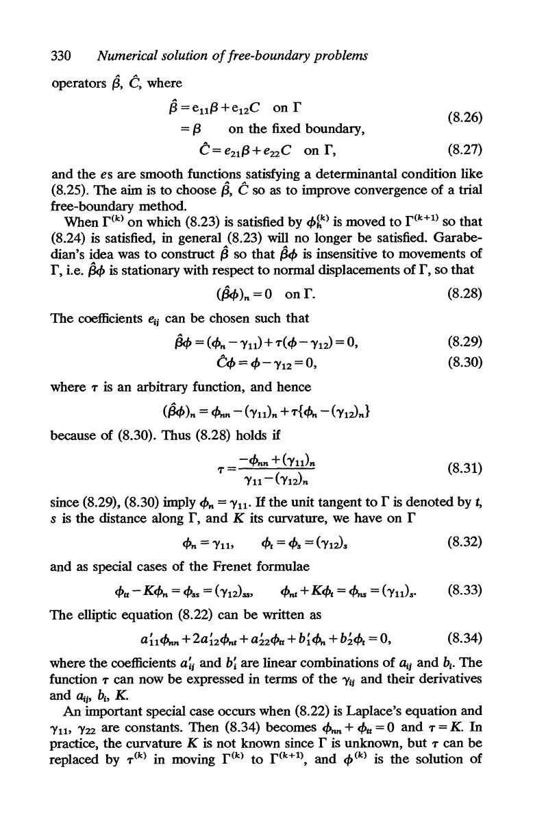
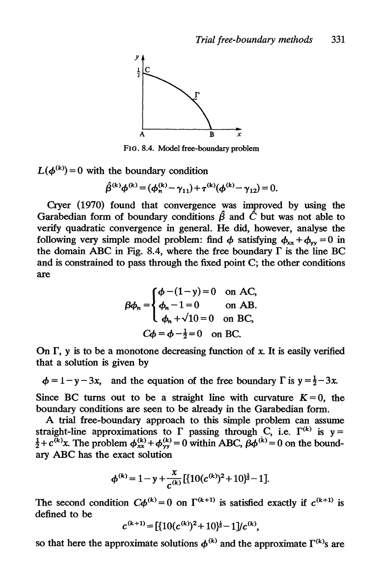
FIG. 8.4. Model free-boundary problem
L(
</>(k)
= 0 with the boundary condition
~(k)</>(k)
=
(</>~k)_
'Y11)+
T(k)(</>(k)_
'Yd
==
O.
Cryer (1970) found that convergence
was
improved by using the
Garabedian form of boundary conditions
~
and C but was not able to
verify quadratic convergence in general.
He
did, however, analyse the
following very simple model problem: find
</>
satisfying
<!>xx
+
</>yy
= 0 in
the
domain
ABC
in Fig. 8.4, where the free boundary r is the line BC
and
is constrained
to
pass through
the
fixed point C; the other conditions
are
{
</>-(l-
Y
)=O
on
AC,
f3<I>n
=
<I>n
- 1 = 0 on AB.
<I>n
+1/'10 = 0 on BC,
Of>
=
</>
-!
= 0 on
Be.
On
r,
Y
is
to
be
a monotone decreasing function of
x.
It
is
easily verified
that a solution is given by
</>
= 1 - Y - 3x, and
the
equation of the free boundary r
is
y
=!-
3x.
Since
BC
turns out
to
be
a straight line with curvature K = 0, the
boundary conditions are seen
to
be
already in
the
Garabedian form.
A trial free-boundary approach
to
this simple problem can assume
straight-line approximations
to
r passing through .C, i.e. r(k)
is
y
==
!+
C(k)X.
The
problem
</>c;2+<I>~~)
= 0 within ABC,
(3<f>(k)
= 0 on the bound-
ary
ABC
has
the
exact solution
</>(k)
=
1-
y +
:)
[{10(c(k)2+
10}!-1].
c
The
second condition
C</>(k)
= 0 on r(k+l) is satisfied exactly
if
C(k+l)
is
defined
to
be
C(k+l) =
[{10(c(k)2+
10}!-l]/c(k),
so that here the approximate solutions
</>(k)
and
the
approximate r(k)s are