Crank J. Free and Moving Boundary Problems
Подождите немного. Документ загружается.

372
Numerical solution
of
free-boundary problems
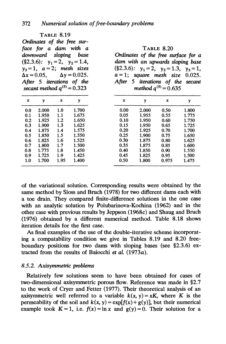
TABLE
8.19
Ordinates
of
the
free
sur-
face
for
a dam with a
downward sloping base
(§2.3.6):
Yl
= 2,
Y2
= 1.4,
Y3
= 1, a = 2; mesh sizes
ax
= 0.05,
ay
= 0.025.
After 5 iterations
of
the
secant method
q(5)
= 0.323
x y x
0.0 2.000 1.0
0.1 1.950
1.1
0.2 1.925 1.2
0.3 1.900 1.3
0.4 1.875 1.4
0.5 1.850 1.5
0.6 1.825 1.6
0.7 1.800 1.7
0.8 1.775 1.8
0.9 1.725 1.9
1.0 1.700 1.95
y
1.700
1.675
1.650
1.625
1.575
1.550
1.525
1.500
1.450
1.425
1.400
TABLE
8.20
Ordinates
of
the
free
surface
for
a
dam with an upwards sloping base
(§2.3.6):
Yl
= 2,
Y2
= 1.3,
Y3
= 1,
a = 1; square mesh size 0.025.
After 5 iterations
of
the secant
x
0.00
0.05
0.10
0.15
0.20
0.25
0.30
0.35
0.40
0.45
0.50
method
q(5)
= 0.635
y
2.000
1.955
1.950
1.950
1.925
1.900
1.875
1.875
1.850
1.825
1.800
x
0.50
0.55
0.60
0.65
0.70
0.75
0.80
0.85
0.90
0.95
0.975
y
1.800
1.775
1.750
1.725
1.700
1.650
1.625
1.600
1.550
1.500
1.475
of the variational solution. Corresponding results were obtained by the
same method by Sloss and Bruch (1978) for two different dams each with
a toe drain. They compared finite-difference solutions in the one case
with an analytic solution by Polubarinova-Kochina (1962) and in the
other case with previous results by Jeppson
(1968c) and Shaug and Bruch
(1976) obtained by a different numerical method. Table 8.18 shows
iteration details for
the
first case.
As final examples of the use of the double-iterative scheme incorporat-
ing a compatability condition we give in Tables 8.19 and 8.20 free-
boundary positions for two dams with sloping bases (see §2.3.6) ex-
tracted from the results of Baiocchi
et al. (1973a).
8.5.2. Axisymmetric problems
Relatively few solutions seem
to
have been obtained for cases of
two-dimensional axisymmetric porous
flow.
Reference was made in §2.7
to
the work of Cryer and Fetter (1977). Their theoretical analysis of an
axisymmetric well referred
to
a variable k(x, y) = xK, where K
is
the
permeability of
the
soil and k(x, y) = exp[f(x)+ g(y)],
but
their numerical
example took K
= 1, i.e. f(x) = In x and g(y) =
O.
Their solution for a
Variational inequality and complementarity methods
373
Baiocchi variable w required the minimization of
J(w)
= L
x(w~+w;+2w)dxdy,
subject
to
boundary conditions discussed in §2.7. Linear finite elements
on
a triangulated domain were used in which, because the solution varies
most rapidly near the well, the subdivisions were taken
to
be uniform in
the y-direction and logarithmic in the x-direction. Thus the coordinates
of the grid points were
Yj=jH/m,
Xj = r exp[(iln)ln(R/r)],
The
integer m was always chosen to
be
a multiple of 4 so that the corner
D was a grid point where w
is
not smooth.
The
Cryer algorithm was used
to
solve the discretized complementarity problem.
The
numerical exam-
ple quoted by Cryer and Fetter (1977) referred to a well of radius r = 4.8
sunk in a soil of depth H
= 48 and radius R = 76.8; the water level in the
well
is maintained by pumping at a constant height
hw
= 12 and the free
boundary meets the wall of the well
at
a height
h".
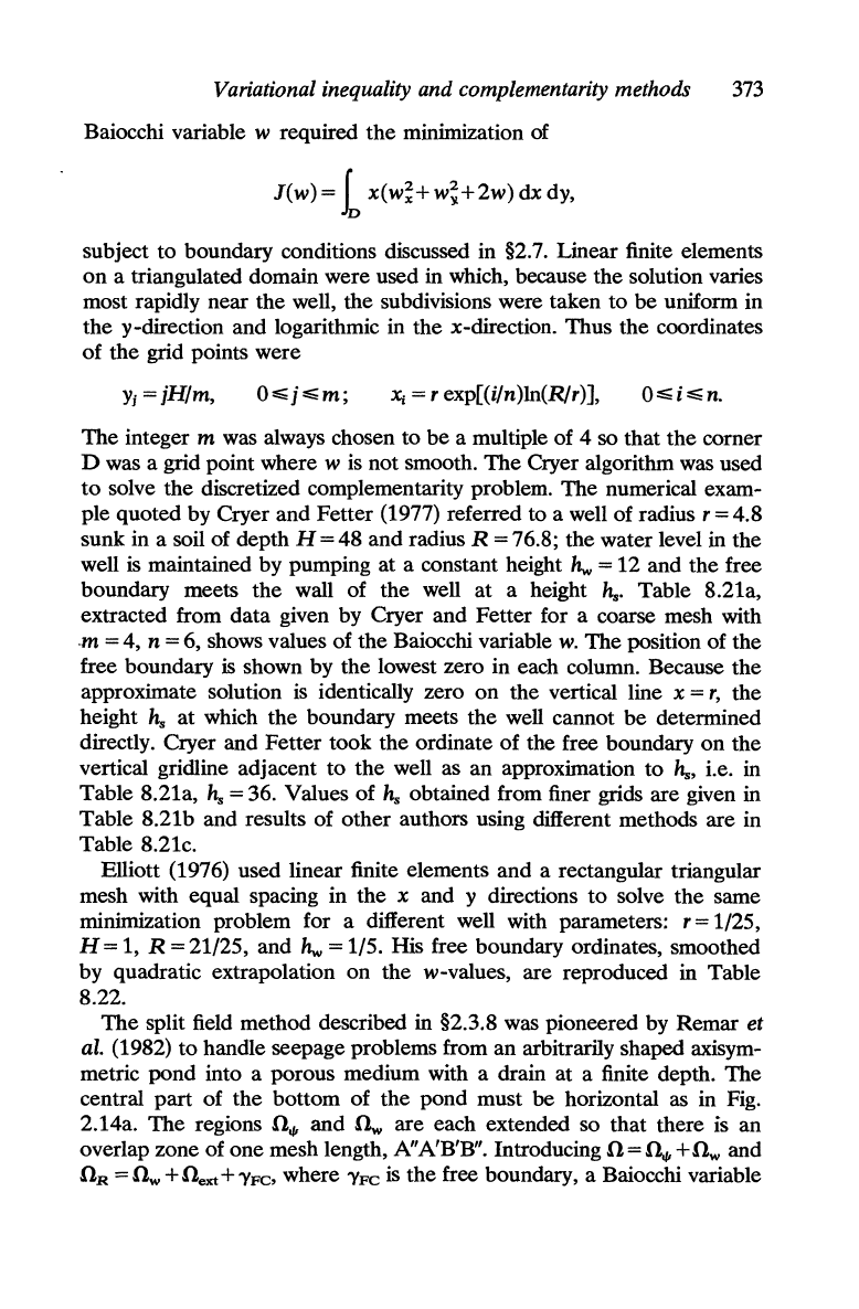
Table 8.21a,
extracted from data given by Cryer and Fetter for a coarse mesh with
-m
= 4, n = 6, shows values of the Baiocchi variable
w.
The position of the
free boundary
is
shown by the lowest zero in each column. Because the
approximate solution
is
identically zero
on
the vertical line x =
r,
the
height
hs
at which the boundary meets the well cannot
be
determined
directly. Cryer and Fetter took the ordinate of the free boundary
on
the
vertical gridline adjacent to
the
well as an approximation to
h",
i.e. in
Table 8.21a,
h"
= 36. Values of
h"
obtained from finer grids are given in
Table 8.21b and results of other authors using different methods are in
Table 8.21c.
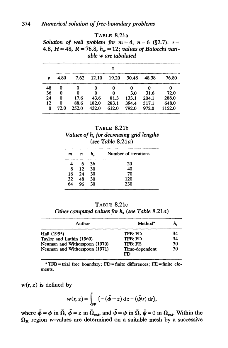
Elliott (1976) used linear finite elements and a rectangular triangular
mesh with equal spacing in the
x and Y directions
to
solve the same
minimization problem for a different well with parameters: r =
1/25,
H = 1, R = 21/25, and
hw
=
115.
His free boundary ordinates, smoothed
by quadratic extrapolation on the w-values, are reproduced in Table
8.22.
The
split field method described in §2.3.8 was pioneered by Remar
et
al. (1982)
to
handle seepage problems from an arbitrarily shaped axisym-
metric pond into a porous medium with a drain at a finite depth.
The
central part of the bottom of the pond must
be
horizontal
as
in Fig.
2.14a.
The
regions
01/1
and
Ow
are each extended so that there is an
overlap zone of one mesh length, A"A'B'B". Introducing
O=~+Ow
and
OR
=
Ow
+
Oext
+
YFC,
where
YFC
is the free boundary, a Baiocchi variable
374 Numerical solution
of
free-boundary problems
TABLE
8.2la
Solution
of
well problem
for
m = 4, n = 6 (§2.7): r =
4.8, H = 48, R = 76.8,
hw
= 12; values
of
Baiocchi vari-
able
ware
tabulated
y
48
36
24
12
0
x
4.80 7.62 12.10 19.20 30.48 48.38
0 0
0 0 0
@
0 0 0
0
3.0 31.6
0
17.6
43.6 81.3 133.1 204.1
0 88.6 182.0 283.1
394.4 517.1
72.0 252.0 432.0 612.0 792.0 972.0
TABLE
8.2lb
Values
of
h.
for
decreasing grid lengths
(see Table
8.2la)
m n h.
4 6
36
8 12 30
16 24 30
32 48 30
64 96 30
Number of iterations
20
40
70
120
230
TABLE
8.2lc
76.80
0
72.0
288.0
648.0
1152.0
Other computed values
for
h. (see Table
8.2la)
Author
Hall (1955)
Taylor and Luthin (1969)
Neuman and Witherspoon (1970)
Neuman and Witherspoon (1971)
TFB:FD
TFB:FD
TFB:FE
Time-dependent
FD
34
34
30
30
a TFB = trial free boundary;
FD
= finite differences;
FE
= finite ele-
ments.
w(r,
z)
is defined by
w(r,z)=
L
{-(<f;-z)
dz-(.frlr)
dr},
where
<f;
=
<f>
in
n,
<f;
= z in
liext,
and
.fr
=
1/1
in
n,
.fr
==
0 in
next.
Within
the
.oR
region w-values are determined
on
a suitable mesh by a successive
Variational inequality
and
complementarity methods
375
TABLE
8.22
Ordinates
of
free surface for
axisym-
metric well for different
mesh
sizes i!lx;
r = 1/25, H = 1, R = 21/25,
hw
= 1/5,
x = 1/25 + i/20
Ax
=
1/10
Ax
=
1/20
Ax=I/40
1
8212
8158
2
8456 8394
8406
3
8610
8620
4
8719 8739
8793
5
8931
8943
6
9056 9076
9084
7
9198
9213
8
9292
9290 9329
9
9427
9435
10
9506
9533 9540
11
9619
9629
12
9658
9699
9719
13
9742 9797
14
9855
9849
9865
15
9934
9931
over-relaxation scheme with projection, sweeping
to
the left along mesh
lines and downwards, starting from the upper right-hand corner.
In
the
n."
region, a successive over-relaxation scheme determines
!/I.
To
deal with the overlap zone,
the
Ow
region is swept to its last internal
vertical mesh line, i = M in Fig. 2.14b, and values of
!/I
are then
calculated along this line from
the
relationship
!/I
= -rw" suitably approxi-
mated by
These
!/IM,i
values provide
the
Dirichlet boundary data for the
01/1
region
in which
the
SOR
solution for
!/I
can now proceed. Values of W
at
i = M
-1,
the
boundary of
the
Ow
region, are then required for the next
stage
of
the
iteration cycle,
the
updating of w-values by
SOR
with
projection in
Ow.
In
the definition of w given above, an integration path
is
chosen which starts vertically downwards from F
to
the
line j
i!lz
being
evaluated and continues horizontally
to
the point
P«M-1)
i!lr,
j i!lz),
leading
to
the approximation
1
(!/IM-l,i
!/IM,i)
WM-l,i=WM,i+2:
M-1
+ M .
The
discharge rate q
is
not known a priori but has
to
be
determined so
376
Numerical solution
of
free-boundary problems
that a compatability condition fh(q)=O is satisfied where fh(q)=
(wq)p-h,
-!h~
and
F-
h2
denotes
the
first mesh point vertically below F.
The
underlying physical assumption is
that
the
velocity of flow is assumed
to
be
zero
at
the
point
F-!h
2
•
The
iterative cycle
is
performed for two
estimated values of q and successive estimates are based
on
the
secant
method. The method will not converge
if
fh(q) becomes negative. Special
formulae for calculating W
on
the
bottom of
the
pond, the choice of an
optimum relaxation parameter and
the
influence of the singularity
on
the
axis r = 0 are discussed by Remar et
al.
(1982). They present numerical
results for several examples and favourable graphical comparisons with
results obtained by Jeppson (1968a,c).
8.6. A
general
algorithm
for partially
unsaturated
flow
Alt (1979, 1980a,b) proposed and used a new algorithm
to
be
applied
to
saturated-unsaturated flow in a medium of any shape which can
be
inhomogeneous and anisotropic for any boundary conditions. We give
here
an
outline of his formulation
on
which
the
algorithm
is
based. More
details of the mathematical properties, theorems, and conditions are given
in Alt's papers.
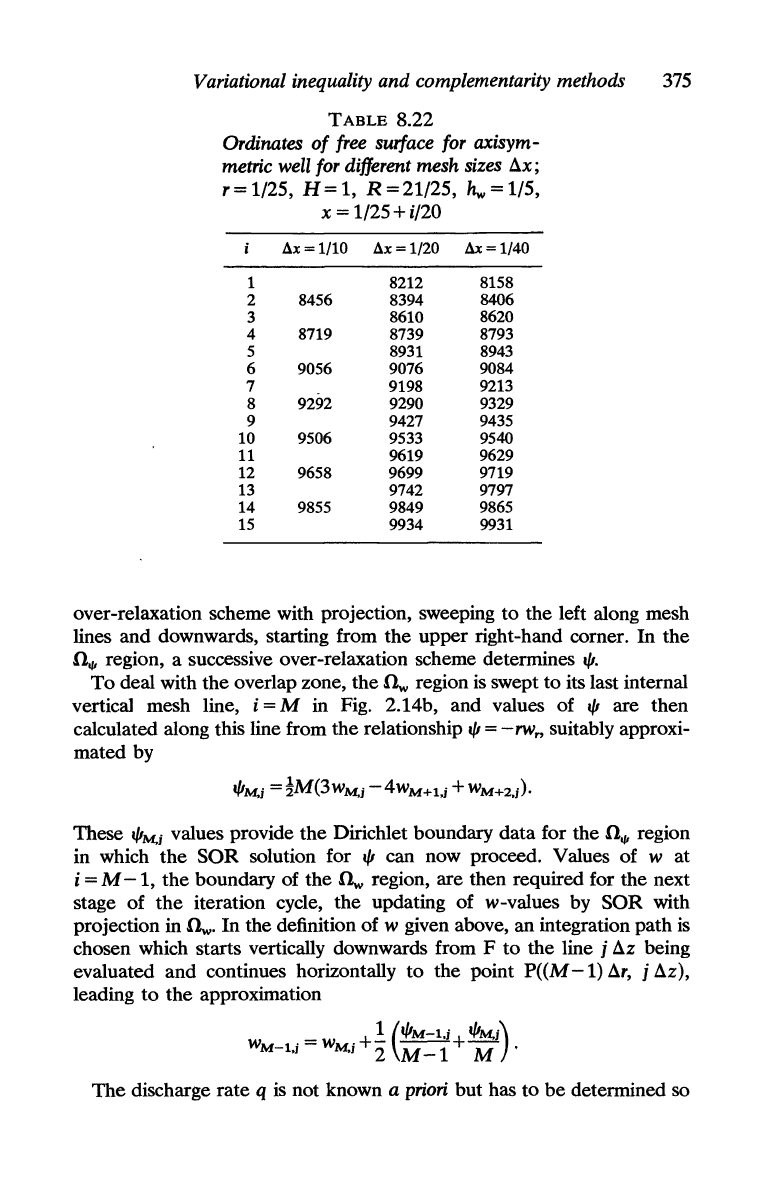
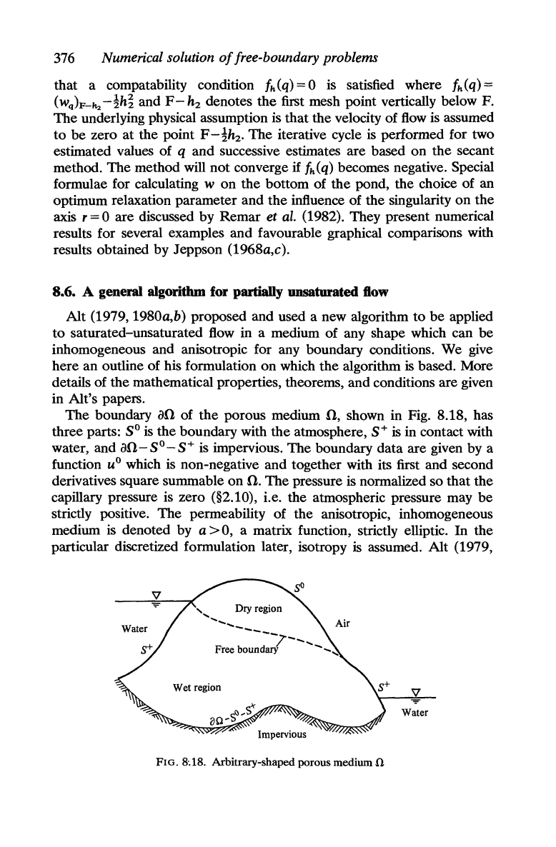
The boundary
ao
of
the
porous medium
0,
shown in Fig. 8.18, has
three parts:
SO
is the boundary with
the
atmosphere, S+ is in contact with
water, and ao-so-s+ is impervious.
The
boundary data are given by a
function
UO
which is non-negative and together with its first and second
derivatives square summable
on
O. The pressure is normalized so that the
capillary pressure is zero (§2.10), i.e. the atmospheric pressure may
be
strictly positive.
The
permeability of the anisotropic, inhomogeneous
medium
is
denoted by a> 0, a matrix function, strictly elliptic. In the
particular discretized formulation later, isotropy
is
assumed.
Alt
(1979,
Water
Water
Impervious
FIG. 8: 18. Arbitrary-shaped porous medium
fi
A general
algorithm
for
partially unsaturated
flow
377
1980a,b) established
that
there
are
functions u
and
'Y
with
X{
(u
>
O)}
"""
'Y
"""
1 which satisfy
the
inequality
fa
\7(v-u)a(\7u+'Ye)~O
(8.98)
for all functions v
where
u
and
v
are
square summable together with their
first
and
second derivatives, v =
UO
on
S+,
V"""
UO
on
So, X is
the
characteristic function, i.e. X = 1, u > 0, X = 0, u = 0,
and
e is
the
vertical
unit
vector in
the
direction
of
gravity.
Alt
(1980a) extended (8.98)
to
include a prescribed flux function
on
part
of
the boundary
to
allow for a
leaky region in
the
base of a dam, for example.
The
assumption
is
that
unsaturated flow is controlled by
an
extension
of
Darcy's law, i.e. q =
-a(\7u
+
'Ye)
so
that
the
inequality (8.98) is equivalent
to
\7
.
[a(\7u
+
'Ye)]
= 0 in
0,
U =
UO
on
S+,
(\7u +
'Ye)
.
v=O
on
ao-so-s+,
u",,"uo,
(\7u+'Ye)'v",,"O
on
So,
(u-UO)(\7u
+
'Ye)
'v=o
on
So,
where
v is
the
unit
outward normal
to
the
relevant surface.
The
function
'Y
is
here
a non-linear function
of
the
degree
of
saturation, which is
characteristic
of
the
porous
medium (Bear 1972, p. 496).
The
case of a
capillary fringe is included
under
uo>O
on
So.
In
a homogeneous medium
the
solution consists only
of
saturated
regions where
u>O
and
'Y=1
and
dry regions where 'Y=O.
Alt
(1979)
proved
that
in these cases
the
inequality \7.
(ae);;;;:O
is always satisfied.
In
the
saturated regions
the
function u is
the
solution
of
an elliptic partial
differential equation.
For
general inhomogeneous media, however,
the
condition \7. (ae)
<0
may hold somewhere
and
then
an unsaturated
region may exist in which 0
<
'Y
<
1.
In
this region u = 0
and
the
flow is
determined by
the
gravitational force
and
not by
the
pressure gradient.
The
function
'Y
is a solution
of
a first-order equation
of
flow.
Alt
(1979)
analyses a simple example
of
an
unsaturated region in a horizontally
stratified inhomogeneous medium with a flow
pattern
closely resembl-
ing
that
shown in Fig. 8.26.
The
physical
signific~nce
of
the
condition
\7
. (ae) < 0 is
that
it permits
the
continuity
of
flow condition
to
be
satisfied between a saturated
and
an
unsaturated region.
Thus
suppose
the
saturated
and
unsaturated regions
lie respectively above
and
below a horizontal surface
on
which
the
permeability changes from
as
in
the
saturated
to
au
in
the
unsaturated
region as in
Alt's
(1979) example
and
as<au.
The
rate
of
flow
to
the
boundary from above is
the
vertical component
of
as
(\7u +
'Yse)
=
qs
where
378 Numerical solution
of
free-boundary problems
"Is
=
1.
The
rate of flow away from the boundary into the unsaturated
medium
is
au
"Iue
=
qu
with
"Iu
<
1.
Continuity of
flow
requires q. =
qu,
which
is
possible if
au>
a.
but not otherwise.
For the discretization, functions
<f>~,
x~
are defined such that
<f>~eHl,2(0)nL""(0),
ieP
h
,
are linearly independent with
<f>~~0
and
L<f>~(x)=l
for
xeOh,
(8.99)
where a sequence of positive numbers
h converges to zero and
Ph
is a
finite set, and
X~
e L ""(0), i e
Ph,
L
x~(x)
= 1 for x e
Oh,
(8.100)
are characteristic functions.
The
corresponding finite-dimensional spaces
of functions are
Hh
=
{V
=
~
vi<f>~,
Vi
real numbers}.
L,. = {"I =
~
"IiX~,
"Ii real numbers}
Boundary data are given
by
u~eHh'
u~~O,
P~,PtcPh
disjoint,
and the corresponding class of admissible functions is
Mh(U~={V
eH
h
,
Vi
=
U~i
for i
ePt,
Vi
~U~i
for i epOJ.
It
is assumed in order
to
prove convergence that the data
0,
So, S+ do
not depend on
h.
A discrete version of the inequality (8.98)
is
introduced
by defining
(8.101)
and imposing the following restrictions:
Hh
contains all linear functions in
Oh,
(8.102)
a~>O
and
e~~O
for
ieP
h
,
(8.103)
a~~O
and
e~~O
for
i,jePhoi'i'j.
(8.104)
Then there
is
a function
Uh
in
Mh(U~
with
u~~O
for i
eP
h
and a function
"IheL,. with
0~"I~~1
with
"I~=1
if
u~>O,
such that
t.
V(v-uh)ah(V~+"Ihe)~O
(8.105)
A general algorithm for partially unsaturated flow
379
Alt's numerical algorithm
is
closely related to
the
existence proof for
(8.105) which
is
as follows. By making use
of
the restrictions (8.102-104)
and inserting (8.101) it is seen
that
(8.105) is equivalent
to
L L
vi(u~a~+'Y~ei!)~O
i j
for every v E Hh and with Vi = 0 for i E
~
and
Vi.;;;;
U~i-
u~
for i
En,
which in turn implies
for
for
i¢PtuP~
or
i
EP~
and
U~<U~i,
i
EP~
and
u~
=
U~i.
(8.106)
Now a new variable
wdi)
=
u~
+
'Y~
is
introduced and
Wh
(i)
~
0 because
of
the
definitions
of
u and
'Y.
The
variables
u,
'Y
are regained through the
expressions
u~
= max(
Wh
(i)
-1,0),
(8.107)
In
order
to
write (8.106) in terms
of
Wh,
the
functions
C~(w),
B~(w)
are
defined by
C~(w)
= L
{(-ai!)max(w(j)-l,
O)+(-e~)min(w(j),
1)}
j""l
(8.108a)
where
i,
j E
Ph.
Then remembering
that
'Y~
= 1
if
i E
Pt
or
e~
= 0, the
existence of
~
and
'Yh
is equivalent to the existence of a vector
Wh
satisfying
Wh(i) =
U~i+
1, i
EPt,
wh(i)=min(u~i+l,B~(wh))'
iEP~
(8.109)
wh(i)=B~(w,.),
i¢~UP~,
where wh(i) are components of
the
vector
Wh
at the points
i.
If
this is written
Wh
=
A~(w),
the
mapping A will
be
continuous and
monotone by (8.104) so that
Wl(i)~W2(i)
implies
A~(Wl)~A~(W2)
for
every
i E
Ph
and fixed points of
Ah
can
be
found by an iterative procedure
if at least
one
solution of
~
can
be
found below and
one
above
the
fixed
point. Because
A~(O)~O,
the
vector
w=O
is
a lower solution and
Alt
(1980b) also established an upper solution of A. This completes the proof
and suggests an iterative numerical algorithm based
on
(8.109).
Alt
(1979, 1980a) showed
that
at
least a subsequence
of
solutions of
the
discrete problem converges
to
a solution
of
the
continuous problem.
380 Numerical solution
of
free-boundary problems
e
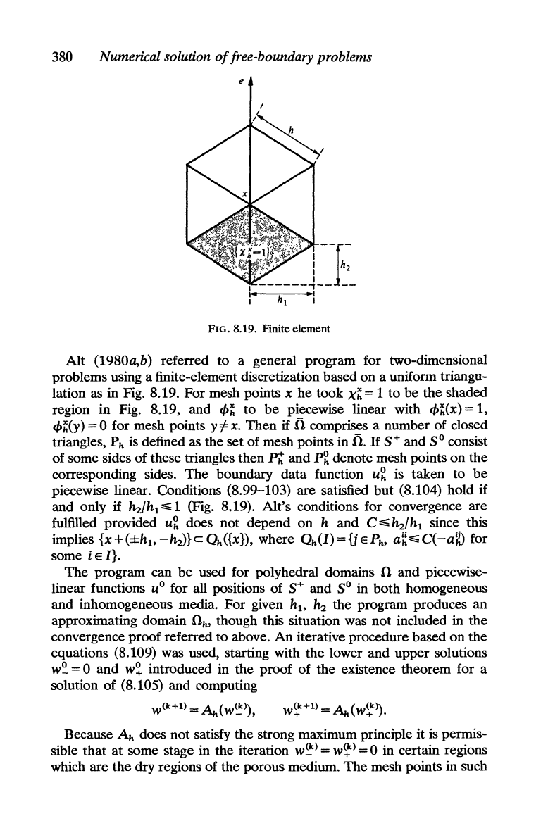
FIG. 8.19. Finite element
Alt (1980a,b) referred
to
a general program for two-dimensional
problems using a finite-element discretization based
on
a uniform triangu-
lation as in Fig. 8.19. For mesh points x he took
Xh=
1
to
be
the
shaded
region in Fig. 8.19, and
q,h
to
be
piecewise linear with
q,h(X)
= 1,
q,h(Y)
= 0 for mesh points Y
1=
x. Then if
fi
comprises a number of closed
triangles,
Ph
is
defined as the set of mesh points in fi.
If
S+ and
SO
consist
of some sides of these triangles then Pt and
~
denote mesh points
on
the
corresponding sides.
The
boundary data function
u~
is taken
to
be
piecewise linear. Conditions (8.99-103) are satisfied
but
(8.104) hold if
and only if
~/hl
z;, 1 (Fig. 8.19). Alt's conditions for convergence are
fulfilled provided
u~
does not depend
on
hand
C
~
~/hl
since this
implies
{x+(±hI>-~}cQ,,({x}),
where Qh(I):;::{jEPh,
a~z;,C(-a~)
for
some
iEI}.
The
program can
be
used for polyhedral domains 0 and piecewise-
linear functions U
O
for all positions of
S+
and
SO
in both homogeneous
and inhomogeneous media. For given
hI>
~
the program produces
an
approximating domain
Oh,
though this situation was not included in
the
convergence proof referred to above. An iterative procedure based
on
the
equations (8.109) was used, starting with
the
lower and upper solutions
w~
= 0 and
w~
introduced in the proof of
the
existence theorem for a
solution of (8.105) and computing
Because
Ah
does not satisfy
the
strong maximum principle it
is
permis-
sible
that
at
some stage in the iteration
w~)
=
w~)
= 0 in certain regions
which are
the
dry
regions of the porous medium.
The
mesh points in such
A general algorithm for partially unsaturated flow
381
S
O.
h'
S
+·
h'
Reservoir
Impervious
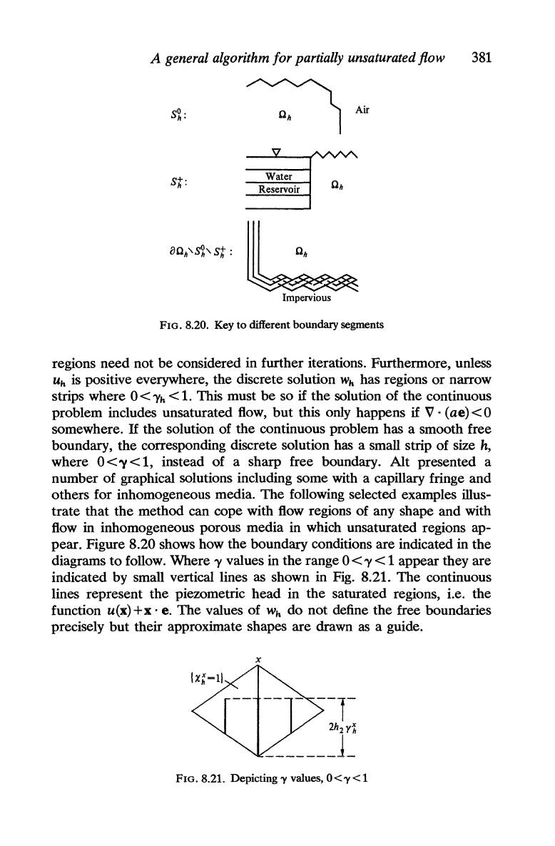
FIG.
8.20. Key to different boundary segments
regions need not
be
considered in further iterations. Furthermore, unless
Uk
is positive everywhere, the discrete solution Wk has regions
or
narrow
strips where 0 <
'Yk
< 1. This must
be
so
if
the
solution
of
the continuous
problem includes unsaturated flow,
but
this only happens
if
V·
(ae)<O
somewhere.
If
the solution of the continuous problem has a smooth free
boundary,
the
corresponding discrete solution has a small strip of size
h,
where
0<'Y<1,
instead of a sharp free boundary. Alt presented a
number of graphical solutions including some with a capillary fringe and
others for inhomogeneous media. The following selected examples illus-
trate that
the
method can cope with flow regions of any shape and with
flow in inhomogeneous porous media in which unsaturated regions ap-
pear. Figure 8.20 shows how the boundary conditions are indicated in the
diagrams
to
follow. Where
'Y
values in the range 0 <
'Y
< 1 appear they are
indicated by small vertical lines as shown in Fig. 8.21.
The
continuous
lines represent
the
piezometric head in the saturated regions, i.e. the
function
u(x)+x'
e.
The
values of
Wk
do not define the free boundaries
precisely
but
their approximate shapes are drawn
as
a guide.
x
--
-
--1-
2h2r~
_______
1_
FIG.
8.2l.
Depicting
'Y
values, 0 <
'Y
< 1