Crank J. Free and Moving Boundary Problems
Подождите немного. Документ загружается.

382
Numerical solution
of
free-boundary problems
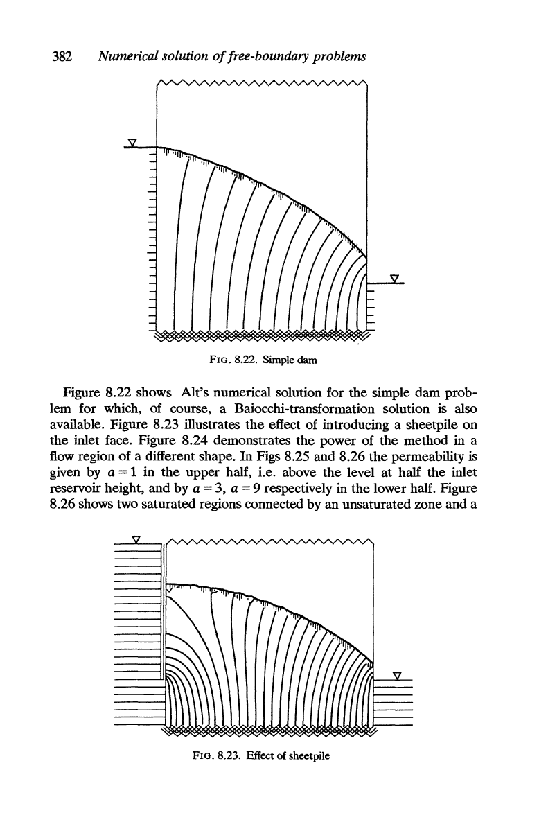
FIG. 8.22. Simple dam
Figure 8.22 shows Alt's numerical solution for the simple dam prob-
lem for which, of course, a Baiocchi-transformation solution
is
also
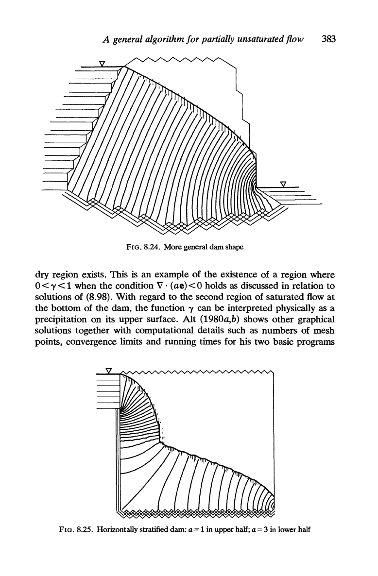
available. Figure 8.23 illustrates
the
effect of introducing a sheetpile
on
the
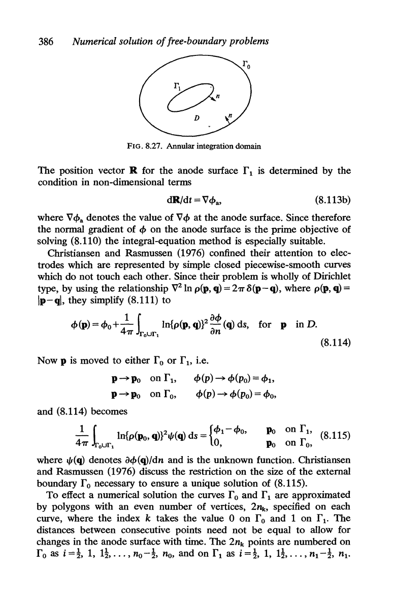
inlet face. Figure 8.24 demonstrates
the
power of
the
method in a
flow region
of
a different shape. In Figs 8.25 and 8.26
the
permeability
is
given by a = 1 in
the
upper half, i.e. above
the
level at half
the
inlet
reservoir height, and by a = 3, a = 9 respectively in
the
lower half. Figure
8.26 shows two saturated regions connected by an unsaturated zone and a
FIG. 8.23. Effect of sheetpile
A general algorithm for partially unsaturated flow
383
FIG. 8.24. More general dam shape
dry region exists. This
is
an example of
the
existence
of
a region where
O<y
< 1 when the condition V . (ae)
<0
holds
as
discussed in relation
to
solutions of (8.98). With regard to the second region
of
saturated flow
at
the
bottom of
the
dam,
the
function y can
be
interpreted physically as a
precipitation on its upper surface. Alt (1980a,b) shows other graphical
solutions together with computational details such as numbers of mesh
points, convergence limits and running times for his two basic programs
FIG. 8.25. Horizontally stratified dam: a= 1 in upper half; a= 3 in lower half

384
Numerical solution
of
free-boundary problems
I§~~~,"
",
:11
',"I'
'I"f
"'.
I , ,
•••
• • • , • I
FIG. 8.26. Horizontally stratified dam: a= 1 in upper half;
a=9
in lower half
one
for inhomogeneous media and a simpler version for homogeneous
media.
8.7. Integral. equation methods
Reference was made in §8.2.1
to
integral equation methods as
one
of
several possible ways of computing trial solutions for successive estimates
of the position of
the
free boundary in trial and
error
methods. Several
references to integral-equation formulations of electrochemical machining
problems were given in §2.12.3.
The
present section contains a brief
general description of
the
numerical solution of Laplace's equation in a
fixed domain by expressing it in
the
form
of
an
integral equation.
Then
some developments in relation
to
problems of electrochemical machining
are
described.
The
integral equation method in two dimensions solves the equation
V2r/J
=
fir/J
+ a
2
r/J
= 0
ax
2
ay2
,
(8.110)
in a plane domain D with a finite boundary, L,
on
each point of which
r/J
or
its normal derivative
ar/J/an
are prescribed.
The
domain may
be
bounded
or
unbounded and simply
or
multiply connected, provided only
that
L must consist
of
closed contours with no cuts
or
cusps.
The
boundary data
are
to
be
piecewise continuous except possibly for jumps
in the normal derivative
ar/J/an
at corners
of
L.
No value need
be
given
at
such points nor
at
other
discrete points where
the
boundary condition
changes.

Integral equation methods
385
The
method
to
be
described starts from Green's formula (the third
identity) in the form
L
{«>'(q)ln
Iq-pl-
«>(q)ln'
Iq-pl}
dq
=
7J(p)«>(P),
(8.111)
where p, q are vectors specifying points of the plane and on L respec-
tively; the prime denotes differentiation at the point q along the inward
normal to the domain and dq
is
the differential increment of L at q.
If
P
is
a point in D then
7J(P)
=
2n,
but
if
p
is
a boundary point on
L,
7J(P)
= O(p), where O(p)
is
the internal angle at the point p, i.e. the angle
between the tangents to L
on
either side of p. In the latter case (8.111)
becomes (Jaswon and Symm, 1977)
L
{«>'(q)ln
Iq-pl-
«>(q)ln'
Iq-pl}
dq
-O(p)«>(P) = 0,
pEL.
(8.112)
This provides a linear relationship between the boundary values of a
solution
«>
of (8.110) and those of its normal derivative. Hence, given
values of either
«>
or
a«>/an
at each point of L
we
have a linear equation
for the other corresponding boundary values,
or
a pair of equations when
«>
is given on a part of L and
«>'
on the remainder. We note that provided
L has no cusps,
7J(p)
is never zero and so by substituting the solution of
(8.112), together with the original boundary data, into (8.111) the value of
«>
at any point p in D and on L can
be
obtained.
Exc~ptions
to the
statement that the integral equation arising from (8.112) has a unique
solution are discused by Jaswon and Symm (1977) and Baker (1979). The
general basis of a numerical procedure for solving the integral equations
is
to
divide the boundary L into smooth intervals such that any comers
or
changes in form of the boundary occur at the points of subdivision. The
functions
«>
and
«>'
are approximated by constant values within each
interval.
The
boundary L itself
is
approximated by a polygon by replacing
each interval by two chords which join its end points to
the
nodal point
within it. A system of simultaneous equations results, in which all the
coefficients of the discretized
«>
and
«>'
can
be
computed analytically.
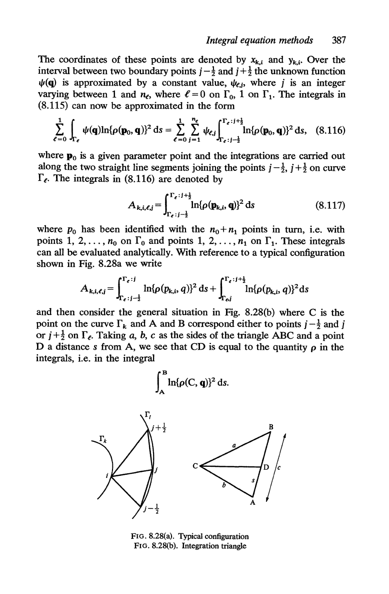
8.7.1. Two-dimensional annular electrochemical machining problem
We now discuss in more detail the integral-equation method of solving
a quasi-steady-state model of the electrochemical machining process
outlined in §2.12.3 used by Christiansen and Rasmussen (1976). Their
system and terminology are illustrated in Fig. 8.27, where
f 0
is
the
cathode and
f 1 the anode and the problem
is
to
find a function
«>
satisfying (8.110) in
the
annular space D subject to boundary conditions
«>
=
«>0
on
fo,
«>
=
«>1
on
fl.
(8.113a)
386
Numerical solution
of
free-boundary problems
FIG. 8.27. Annular integration domain
The
position vector R for the anode surface f I is determined by the
condition in non-dimensional terms
dR/dt
= V
cf>a,
(8. 113b)
where V
cf>a
denotes the value
of
V
cf>
at the anode surface. Since therefore
the normal gradient of
cf>
on
the anode surface
is
the
prime objective of
solving (8.110) the integral-equation method
is
especially suitable.
Christiansen and Rasmussen (1976) confined their attention to elec-
trodes which are represented by simple closed piecewise-smooth curves
which do not touch each other. Since their problem
is
wholly of Dirichlet
type, by using the relationship V2ln p(p, q) = 2'IT5(p-q), where p(p, q) =
Ip-ql,
they simplify (8.111) to
1 i
acf>
cf>(P)
= cf>o+4 In{p(p,
q)fa-
(q)
ds, for p in D.
'IT
our
l
n
Now P is moved to either f 0
or
f
1>
i.e.
P~Po
on
f1>
P~Po
on fo,
and (8.114) becomes
cf>(p)
~
cf>(Po)
=
cf>b
cf>(p)
~
cf>(Po)
=
cf>o,
(8.114)
4
1 f In{p(po,q)ft/l(q) ds =
{cf>OI-cf>O,
Po
on
f1>
(8.115)
'IT.lrourl
,Po
onfo,
where
t/I(q)
denotes
acf>(q)/dn
and
is
the unknown function. Christiansen
and Rasmussen (1976) discuss the restriction
on
the size
of
the external
boundary f 0 necessary to ensure a unique solution of (8.115).
To
effect a numerical solution the curves f 0 and
flare
approximated
by polygons with an even number of vertices,
2l1rc,
specified
on
each
curve, where the index k takes the value 0
on
fo
and 1 on
fl'
The
distances between consecutive points need not
be
equal to allow for
changes in the anode surface with time. The 2nk points are numbered
on
fo
as
i
=t,
1, It, ... ,
no-t,
no,
and
on
fl
as i
=t,
1, It, ... ,
nl-t,
nl'
Integral
equation methods
387
The
coordinates of these points are denoted by
Xk,i
and
Yk,i'
Over the
interval between two boundary points
j-!
and
j+!
the unknown function
I/I(q)
is
approximated
by
a constant value,
I/II'J'
where j
is
an integer
varying between 1 and
ne,
where t = 0
on
f
0,
1
on
f
l'
The integrals in
(8.115) can now
be
approximated in the
fonn
1 r
l"e
rr
'j+!
l'~o.lre
l/I(q)ln{p{Jlo,qWds =
I'~Oi~
I/Il"i.lre:;_!
In{p(po,
qW
ds, (8.116)
where
Po
is a given parameter point and
the
integrations are carried
out
along the two straight line segments joining the points j
-!,
j +!
on
curve
fl"
The integrals in (8.116) are denoted by
(8.117)
where
Po
has been identified with the
no
+
n1
points in turn, i.e. with
points 1, 2,
...
,
no
on
fo
and points 1, 2,
...
,
nl
on
fl'
These integrals
can all
be
evaluated analytically. With reference
to
a typical configuration
shown in Fig. 8.28a we write
Ak,i,l'J = rre:i 1
In{pCPk.i>
q)}2
ds +
rr~:j+!ln{p(Prc,i>
q)}2ds
Jr
e
:J-2
Jr
eJ
and then consider the general situation in Fig. 8.28(b) where C
is
the
point
on
the curve f k and A and B correspond either to points j
-!
and j
or
j +!
on
fl"
Taking
a,
b,
c as the sides of the triangle
ABC
and a point
D a distance s from
A,
we see
that
CD
is
equal to the quantity p in the
integrals, i.e. in the integral
f:
In{p(C,
qW
ds.
C~-----f
FIG.8.28(a). Typical configuration
FIG.8.28(b). Integration triangle
B

388
Numerical solution
of
free-boundary problems
The
cosine rule gives
p2=s2+b
2
+s(a
2
-b
2
-c
2
)/c, from which we get
J
(
a2-b2-c2)
d
2cs+a
2
-b
2
-c
2
p2
ds =
s+
In
p2+-
tan
-1 2s,
2c c d
where
d={[(a+bf-c
2
][c
2
-(a-b)2]}!
and eventually
I
c
a2-b2+c2
-a
2
+b
2
+c
2
Inp
2
ds=
Ina
2
+
lnb
2
o 2c 2c
d
-1
d
+-tan
2 b
2
2
-2c.
c a +
-c
As j assumes successively the values between 1 and
ne,
the different
distances appear in cyclic order as the quantities
a,
b,
c,
and so lead to a
fast numerical procedure as Christiansen and Rasmussen observe.
Finally, an algebraic approximation to the integral equation (8.115) can
be
written as
i = 1, 2,
...
,
no,
where
k =
1,
k=O
i = 1,
2,
...
,
nh
(8.118)
The system of linear equations was solved by a standard routine. From
values of
acp/an
at points
on
the
anode surface
Vcpa
can
be
determined
and used in a finite-difference form of (8.113b), i.e.
(8.119)
to
determine the new anode shape
at
time (n +
1)
at.
Details were given
by Christiansen and Rasmussen (1976), who checked their procedure by
applying it to the case of two concentric circular electrodes with non-
dimensional radii
Co
and
Ch
C1
<
co,
for which the exact solution
is
(8.120)
On
the interior anode surface
acp)
CP1
-
CPo
ar
r=c,
C1ln(c1/CO)'
(8.121)
When N =
no
=
n1
=
24
and
the
exterior curve
is
far from the critical one
mentioned above
(co
= 1), the values of
acp/an
for
CPo
= 0,
CP1
= 1 are in
Integral equation methods
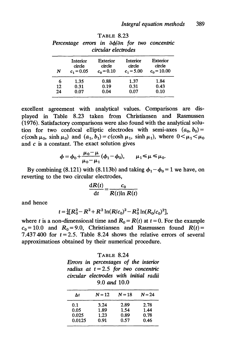
389
TABLE
8.23
Percentage
errors
in
ac/>/an
for
two
concentric
circular electrodes
Interior
Exterior Interior Exterior
circle circle circle circle
N C
1
=0.05
c
o
=0.10
C
1
=5.00
Co=
10.00
6 1.35
0.88
1.37
1.84
12 0.31
0.19 0.31
0.43
24 0.07
0.04 0.07 0.10
excellent agreement with analytical values. Comparisons are dis-
played in Table 8.23 taken from Christiansen and Rasmussen
(1976). Satisfactory comparisons were also found with the analytical solu-
tion for two confocal elliptic electrodes with semi-axes
(ao, b
o
)
=
c(cosh
""'0,
sinh
""'0)
and (al> b
1
)
=
c(cosh""'l>
sinh
""'1),
where 0<""'1
<""'0
and c
is
a constant.
The
exact solution gives
By combining (8.121) with (8.113b) and taking
c/>1-c/>0=
1 we have, on
reverting to the two circular electrodes,
dR(t)
Co
--=--"---
dt
R(t)ln
R(t)
and hence
t
=*[R~-
R2+
R2In(R/co?-
R~
In(Ro/co)2],
where t
is
a non-dimensional time and
Ro
=
R(t)
at t =
O.
For the example
Co
= 10.0 and
Ro
= 9.0, Christiansen and Rasmussen found
R(t)
=
7.437400 for t = 2.5. Table 8.24 shows the relative errors of several
approximations obtained by their numerical procedure.
TABLE
8.24
Errors in percentages
of
the interior
radius
at
t = 2.5 for two concentric
circular electrodes with initial radii
9.0
and
10.0
t:.t
N=12 N=18
N=24
0.1 3.24 2.89 2.78
0.05 1.89 1.54
1.44
0.025 1.23 0.89 0.78
0.0125
0.91
0.57 0.46

390 Numerical solution
of
free-boundary problems
Further satisfactory comparisons were made with a perturbation solu-
tion obtained by Rasmussen and Christiansen (1976) for an elliptical
anode placed symmetrically inside a circular cathode.
In
this problem the
non-dimensional radius of the cathode
is
10.0 and the semi-axes of the
anode are 9.5 and 9.0. Rasmussen and Christiansen (1976) considered
0.25 sin
28
to be a small perturbation on the circle with radius 9.25. The
same problem was studied by Crowley (1979) (see §6.2.7(i)) and
by
Elliott (1980) (see §2.12.3) and all four sets of results are collected
together in Table 8.25 taken from Elliott (1980). Both Crowley and
Elliott make the point that this
is
not an ideal example for fixed-domain
methods
as
the amplitude of oscillation
is
small compared with reasonable
mesh sizes
5r.
They both started from a sinusoidally perturbed anode.
Nevertheless the comparisons are good, especially for the average radius.
The original papers give results for different mesh sizes and for other
machining problems.
Hansen (1980,1983) extended and modified the method of Christian-
sen and Rasmussen (1976) just described in axial symmetry. The elec-
trode surfaces are assumed
to
be axially symmetric and concentric; the
cathode
is
finite and the anode infinite in extent. Each electrode surface
TABLE
8.25
Comparison
of
results for elliptic anode inside circular cathode
Time
c·
CRa
Rca
Ea
~r=0.0625
2N=48
2N=48
~r=0.125
~8
=
'rT/20,
~t
= 0.01
8t=0.025
~8='rT164
Average radius
0.0 9.25 9.25
9.25 9.25
0.5 8.719 8.71
8.727
8.722
1.0 8.320 8.34
8.356 8.351
1.5
8.031 8.03
8.048
8.045
2.0 7.781 7.76 7.778 7.776
2.5 7.531 7.52 7.533 7.532
3.0 7.29
7.307
7.304
3.5 7.08
7.095
7.093
Amplitude of oscillation
0.0 0.25
0.25 0.25 0.025
0.5 0.156 0.15
0.151 0.147
1.0 0.117 0.11
0.118
0.121
1.5
0.094
0.10 0.100 0.095
2.0 0.094
0.09 0.089 0.087
2.5 0.094 0.08
0.080 0.079
3.0
0.07 0.074
0.074
3.5 0.07
0.069
0.066
·C=Crowley
(1979), enthalpy; CR=Christiansen and Rasmussen (1976),
integral equation, numerical;
RC
= Rasmussen and Christiansen (1976), pertur-
bation; E = Elliott (1980), variational inequality;
2N
= number of points on each
electrode.

Integral equation methods 391
may consist of ring-shaped regions in which either Dirichlet or Neuman
type boundary conditions apply. There may be a finite number of circular
common edges where the tangent planes to the surfaces meet
at
an
exterior angle
(3,
O:so;
(3
:so;
2'lT.
The unions of the generators of the regions
on the cathode surface where the Dirichlet condition
is
cf>
=
cf>c
are
denoted by Ceo, and those with the Neuman condition,
acf>/aN
= 0, by
CCN'
The
corresponding notation for the regions of the anode surface
is
CAD
and
CAN'
For
the cylindrical symmetry the appropriate fundamental solution can
be
written
(8.122)
where r has coordinates
r,
z and those of r' are
r',
z', R =
{(
r + r')2 + (z - z 'f}!, and K is the elliptic integral of the first kind. By
using
(8.122) and proceeding from Green's second identity in the usual
way
we
obtain
cf>(r')
-1
= 1 G
acf>
ds
-1
aG
(cf>
-1)
ds -
J.
aG
cf>
ds.
CAD+Cco
aN
CAN
aN
Co.
aN
We now derive an integral equation by taking r' to be a point on the
boundary and using the boundary conditions. We express it
as
Ie
B(s',
s)y(s) ds + v(s')y(s') = u(s'), (8.123)
where C is the union of all the boundaries, i.e. C =
CeoUCCNUCADUC
AN
and s the arc length along
C.
The
functions in
(8.123) are defined by
{
G(r',
r)r,
B(s',s)=
_aG(r'r)r
aN
' ,
where
r=r(s),
r'=r(s'),
Ceo and
CAD
are the closures of Ceo and
CAD
respectively, and a/aN denotes differentiation in the direction of the
inward normal to the surface;
{
acf>/aN,
y(s)=
cf>-1,
cf>,
v(s') =
{~((3/'lT)-l'
u(s') = { 0,
-1,
rECeoUC
AD
,
rEC
AN
,
rECCN;
r'
E
CeoUC
AD
,.
r'ECCNUC
AN
'
rECADUC
AN
,
rECeoUC
CN
·