Crank J. Free and Moving Boundary Problems

352

Numerical solution

of

free-boundary problems

separation line are simultaneously iterated in each loop until a con-

vergence limit is achieved and then the highest mesh point

on

each z-line

on

the plane

A'N'P'G'

at

which x = .J(b

2

-

Z2)

provides

the

best approxi-

mation

to

the

separation that can

be

obtained directly from the finite-

difference mesh.

Numerical experiments show

that

the

iterative process may

not

con-

verge

or

may

be

very slow for arbitrarily chosen starting values for

x.

As

in the two-dimensional problem,

the

initial values of x in

the

free surface

were taken

to

be

linear interpolates between x = .J(b

2

-

Z2)

on

the

line

CL'

in Fig. 8.11 and x = .J(a

2

-

Z2)

on

A'G'

along constant z-lines.

On

each constant y-plane,

the

initial values of x

at

internal mesh points were

obtained by parabolic interpolation along each constant z-line, between

the known values of

x

on

the

surface

D'N'CA'G'L'P'M'

and

the

known

values

at

corresponding points

on

the

surfaces

A'E'FG'

and

G'L'P'M'F

with the additional condition that

acf>/ax

was taken

to

be

zero

on

the

latter

two faces. These parabolic starting values satisfy

the

physical condition

that

acf>/ax

must increase negatively

as

x increases in this problem.

An

initial estimate of

the

shape

of

the surface

M'P'G'F

in Fig. 8.11

on

which

x = 0 is also needed, having in mind that in this surface

the

physical

condition

at

G in

the

free surface, which is

the

cf>-y

plane in Fig. 8.11, is

acf>/az

=

O.

Therefore,

the

intersection of

the

face

M'P'G'F

and

the

free

surface is assumed initially

to

be

a parabola (z -

a)2

=

y(H

-

cf»,

with y

chosen so that

cf>

=

<h,

the value of

cf>

at

the

initial position of L'

on

the

separation line, i.e.

(b-af=y(H-q,J.

The

same parabola can

be

used

between

the

lines M'P' and

FG'

on

each constant-y plane

to

estimate

initial z-values

on

the

whole face

M'P'G'F

by taking

y'to

be

given

by

(b-a)2=y(H-h).

Along L'P',

z=b.

The

formulation

of

this problem in cartesian coordinates

X,

y,

z was

done in order

to

explore

the

feasibility of

the

variable-interchange

technique in three dimensions.

In

fact,

the

problem has cylindrical sym-

metry and Laplace's equation for

cf>

in

the

form

a

2

cf>

1

acf>

a

2

cf>

-+--+-=0

ar2

r

ar

ay2

(8.82)

is appropriate. Boadway

(1976) interchanged

the

variables r and

cf>

and

obtained

the

equation for r = r(

cf>,

y)

to

be

a

2

r

(~)2

+ a

2

r {1+(ar)2}

-2~~

ar

_.!

(~)2

=0.

(8.83)

ay2

acf>

acf>2

!}y

acf>

ay

acf>

ay r

acf>

Ozis (1981) followed

the

treatment

of

eqn (8.61) above with boundary

conditions expressed in cylindrical coordinates

to

obtain numerical solu-

tions of

(8.83).

For

a particular cylindrical dam as shown in Fig. 8.10, in

Methods using variable interchange

353

which a = 1, b = 5/3, H =

1,

h = 1/6, results obtained by the three-

dimensional algorithm in

x,

y,

z coordinates with

&f>

= 5y = 1/12 and

5z = 1/15 compared favorably with those for

the

cylindrical formulation

(8.83).

No formal study

of

the convergence of the iterative solution of the

non-linear finite difference equations proved possible. Instead, Ozis

(1981) quoted numerical experiments which demonstrated reasonable

convergence of some

of

the

numerical values obtained for the three-

dimensional formulation including the position of the free surface, start-

ing from parabolically interpolated x-values.

About

100 iterative cycles

were necessary

to

satisfy a convergence limit

of

Ix;:t,!-xu,kl.;;;10-

3

•

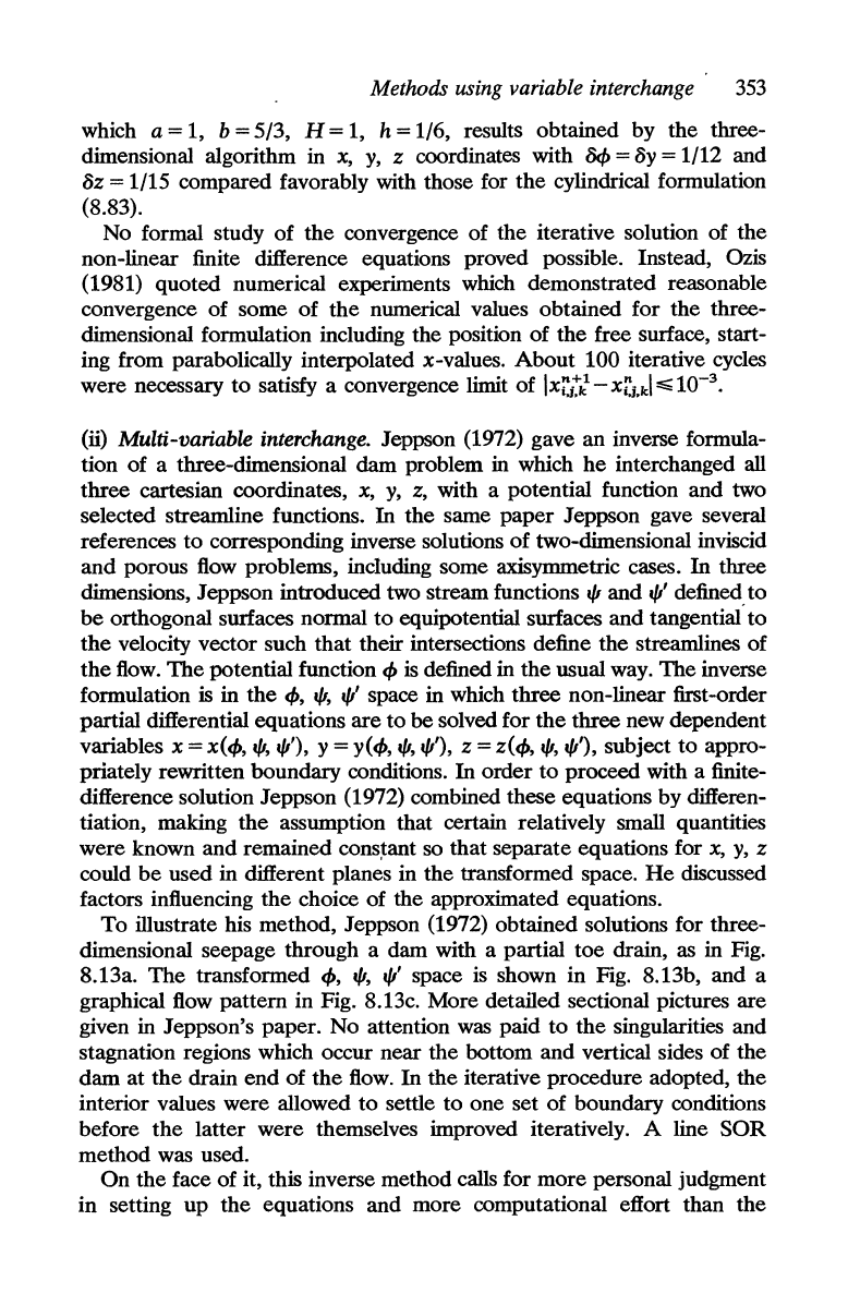
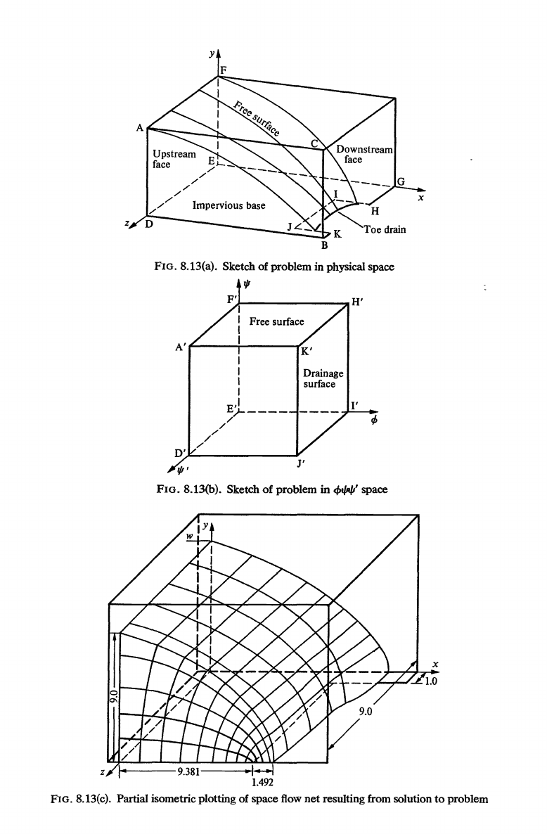
(ii) Multi-variable interchange. Jeppson (1972) gave an inverse formula-

tion

of

a three-dimensional dam problem in which

he

interchanged all

three

cartesian coordinates, x,

y,

z,

with a potential function and two

selected streamline functions.

In

the same paper Jeppson gave several

references to corresponding inverse solutions

of

two-dimensional inviscid

and porous flow problems, including some axisymmetric cases.

In

three

dimensions, Jeppson introduced two stream functions

1/1

and

1/1'

defined

to

be

orthogonal surfaces normal to equipotential surfaces and tangential'to

the

velocity vector such

that

their intersections define the streamlines of

the

flow.

The

potential function

</>

is

defined in

the

usual way.

The

inverse

formulation

is

in the

</>,

1/1,

1/1'

space in which three non-linear first-order

partial differential equations

are

to be solved for

the

three new dependent

variables

x =

x(</>,

1/1,

1/1'),

y =

y(</>,

1/1,

1/1'),

Z =

z(</>,

1/1,

1/1'),

subject to appro-

priately rewritten boundary conditions.

In

order

to

proceed with a finite-

difference solution Jeppson (1972) combined these equations by differen-

tiation, making the assumption that certain relatively small quantities

were known and remained

cons~ant

so

that

separate equations for

x,

y,

z

could

be

used in different planes in the transformed space.

He

discussed

factors influencing the choice of the approximated equations.

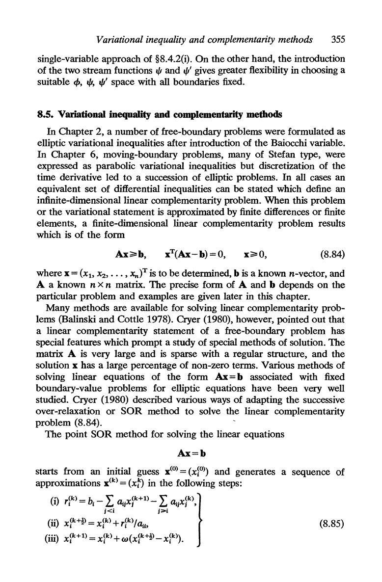
To

illustrate his method, Jeppson (1972) obtained solutions for three-

dimensional seepage through a dam with a partial toe drain, as in Fig.

8.13a.

The

transformed

</>,

1/1,

1/1'

space

is

shown

in

Fig. 8.13b, and a

graphical

flow

pattern in Fig. 8.13c. More detailed sectional pictures are

given in Jeppson's paper. No attention was paid

to

the singUlarities and

stagnation regions which occur near the bottom and vertical sides of the

dam

at

the

drain

end

of

the

flow.

In

the iterative procedure adopted, the

interior values were allowed

to

settle

to

one set

of

boundary conditions

before

the

latter were themselves improved iteratively. A line

SOR

method was used.

On

the face of it, this inverse method calls for more personal judgment

in

setting

up

the equations and more computational effort than the

/

//

/

;>---

///

Impervious base

z D

B

FIG. 8.13(a). Sketch of problem in physical space

'"

A'~---:----~K'

///

I

E;L----

/

Drainage

surface

D'~'~

________

¥

rp'

J'

FIG. 8.13(b). Sketch

of

problem in

cf,t{It/J'

space

FIG.

8.

13(c). Partial isometric plotting

of

space

flow

net resulting from solution

to

problem

Variational inequality and complementarity methods

355

single-variable approach

of

§8.4.2(i).

On

the

other

hand,

the

introduction

of

the

two

stream

functions

t/I

and

t/I'

gives greater flexibility in choosing a

suitable

lb,

t/I,

t/I'

space with all boundaries fixed.

8.S. Variational ineqnality and complementarity methods

In

Chapter

2, a

number

of

free-boundary problems were formulated as

elliptic variational inequalities after introduction of

the

Baiocchi variable.

In

Chapter

6, moving-boundary problems, many

of

Stefan type, were

expressed as parabolic variational inequalities

but

discretization

of

the

time derivative

led

to

a succession

of

elliptic problems.

In

all cases

an

equivalent

set

of

differential inequalities can

be

stated

which define an

infinite-dimensional linear complementarity problem.

When

this problem

or

the variational statement

is

approximated by finite differences

or

finite

elements, a finite-dimensional linear complementarity problem results

which is

of

the

form

Ax;;;;:b,

(8.84)

where

x =

(Xl>

~,

•••

, x,.)T is

to

be

determined, b is a known n-vector, and

A a known n x n matrix.

The

precise form of A and b depends

on

the

particular

problem

and

examples

are

given later in this chapter.

Many methods

are

available for solving linear complementarity prob-

lems (Balinski

and

Cottle 1978). Cryer (1980), however, pointed

out

that

a linear complementarity statement

of

a free-boundary problem has

special features which

prompt

a study

of

special methods

of

solution.

The

matrix A is very large

and

is

sparse with a regular structure, and

the

solution x has a large percentage

of

non-zero terms. Various methods

of

solving linear equations

of

the

form

Ax

= b associated with fixed

boundary-value problems for elliptic equations

have

been

very well

studied.

Cryer

(1980) described various ways

of

adapting

the

successive

over-relaxation

or

SOR

method

to

solve the linear complementarity

problem (8.84).

The

point

SOR

method

for solving

the

linear equations

Ax=b

starts from an initial guess

x(O)

=

(x~O)

and

generates a sequence

of

approximations

X(k)

=

(xf)

in

the

following steps:

(i)

r~k)

= b

i

-

L tl;jX}k+1) - L tl;jX}k)

'}

j<i

j;a.i

(ii)

X~k+!)

=

Xfk)

+

r~k)

I tl;b

(iii)

Xfk+l)

=

X~k)

+

w(X~k+!)-

Xfk).

(8.85)

356

Numerical solution

of

free-boundary problems

The

over-relaxation parameter w

is

a fixed constant and

A=.(tl;j),

b =

(b

i

).

There

is

the well-known theorem that

if

A

is

positive definite the

point

SOR

method converges for all initial guesses

x(O)

if

and only

if

0<w<2.

A natural extension with the linear complementarity (8.84) in mind

is

to

extend (8.85) to the successive steps

(

i)

lk)

=

b.

-

""

n

..

x~k+l)

-

""

n··x~k)

1

'i.J-tJ

J

/""-'1

J ,

j<i

j;;=i

(ii) X[k+1) =

X~k)

+

r[k)

/

tl;b

(iii)

X~k+~

=

X~k)

+

W(X[k+i>

-

X[k»,

(iv)

X~k+l)

=

max(O,

x[k+~».

(8.86)

This

is

the point

SOR

with projection which, provided A is positive

definite, is known to converge for all initial guesses

x(O)

if

and only

if

0<w<2.

The

convergence theorem was proved by Cryer (1971a) after

the method had been used heuristically for a long time starting with

Christopherson and Southwell

(1938).

The

point

SOR

with projection

is

often referred to as the Cryer algorithm. A convergence theorem for

semi-definite matrices A was considered by Glowinski

(1971) and

Eck-

hardt (1975). When w = 1 we have in (8.86) a point Gauss-Seidel

method which Cryer

(1980) equates

to

the problem of finding X[k+1)

which minimizes the quadratic form

!;(X;)

=J(X~k+~),

X~k+1),

•••

,

x~~tl),

x;,

x~~t

•••

,

x~»

over the non-negative real numbers X;, where

J(x)=!xTAx-bTx,

(8.87)

and gives several references

to

studies of this algorithm. Mangasarian

(1977) gave a generalized point

SOR

with projection algorithm for the

solution of symmetric linear complementarity problems and examined its

convergence properties.

In

the point

SOR

method each equation is temporarily satisfied

or

over

satisfied by changing one component

of

the solution vector.

In

a block

SOR

method the equations for a selected group of points

or

components

are solved simultaneously, with other values kept constant for the time

being. The corresponding block

SOR

with projection can

be

written

(i)

~k)

= Bi - L

~j~k+1)

- L

Aij~k),

j<i

j;oi

(ii)

~iK;k+i)

=

~iK;k)

+

~k),

(iii)

K;k~

=

X~k)

+ w(K;k+l) - K;k»,

(iv)

xf

k

+1)

=

Pi(K;k~»,

(8.88)

Variational inequality and complementarity methods

357

where the positive-definite matrix A

is

partitioned into A =

(~j),

where

Au

is

square; x = (X;)

and

b = (BI) are corresponding partitions of x and b.

In

order

to

define

the

projection operator

PI

a factorization of

R"

=

~l

Ri"

is

used where Au is an

N;

xN;

matrix and

Bi>

X; are N;-vectors,

and correspondingly

R~

= IIi'

R~',

where

R~

is the positive orthant. Then

P

+ implies R

N

,

is projected into

R~·.

Cryer (1980) gave different detailed

interpretations of

Pi

and a list of authors who studied them.

The

standard

implementation of

the

algorithm (8.88) performs steps (i), (ii), and (iii)

without imposing non-negativity and finally the projection of step

(iv)

is

performed.

A modified block

SOR

algorithm due to Cottle (1979), Cottle et

al.

(1978) proceeds in a different order

as

follows:

(i)

Solve the linear complementarity problem

A

.~k+fl:;;;.C"~k)=B._

~

A

..

~k+l)_

~

A ..

~k)

.t"1i,Ai

'-'i

'~'J

J

~

ESiJ J ,

j<1

i""l

x~k+fl

:;;;.0,

(X~k+!))T(~I~k+!)

- elk)) = 0,

(8.89)

(ii)

~k+l)

=

~k)

+

Wlk+l)(~k+~

_

~k)),

where

wl

k

+1)

=max{w

:O<w

<wand

Xi

k

)+

w(X<k+!)-

~k)):;;;.O}.

Cottle et

al.

(1978) proved

that

for A positive definite their modified

block

SOR

algorithm converges for

0<w<2.

Cryer (1980) referred

to

other

authors for earlier work on different ranges

of

w.

Since

the

modified

algorithm requires

the

solution of a complementarity problem at every

iteration it looks potentially inefficient in general. However, Cottle and

Sacher (1977) produced a very efficient algorithm for free-boundary

problems in which

the

matrices

~i

are often tri-diagonal M-matrices, i.e.

(l;j:S;;O for

i=!=

j and

A-I

exists and is non-negative. They demonstrated

their

algorithm through the following example, which

is

also reproduced

by Cryer (1980).

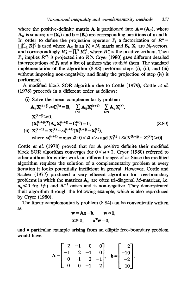
The

linear complementarity problem (8.84) can

be

conveniently written

as

w=Ax-b,

w*,O,

and

a particular example arising from an elliptic free-boundary problem

would have

[

-~

A=

o

-~

~]

=[-1~]

-1

2

-1

,b

-2·

o

-1

2 10

358

Numerical solution

of

free-boundary problems

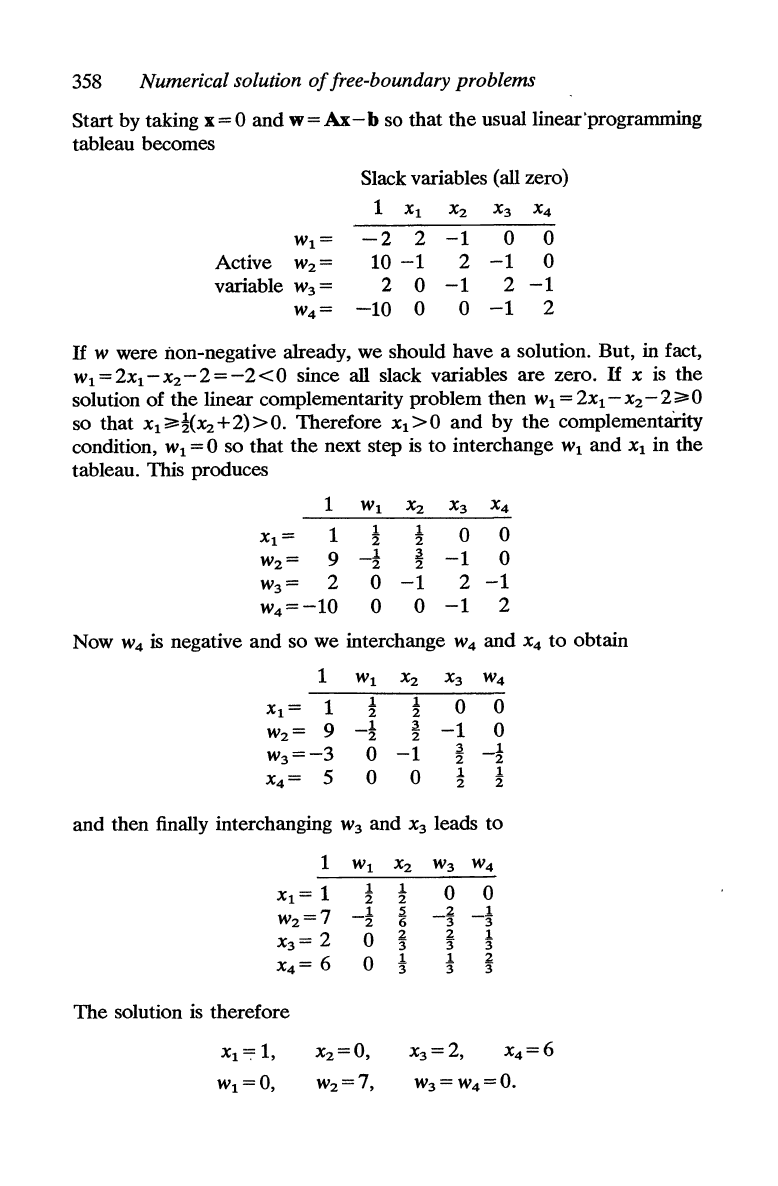
Start by taking

x=O

and

w=Ax-b

so that

the

usuallinear'progranuning

tableau becomes

Slack variables (all zero)

1

Xl

X2

X3 X4

W

l

=

-2

2

-1

0 0

Active

W2=

10

-1

2

-1

0

variable

W3

=

2

0

-1

2

-1

W4=

-10

0 0

-1

2

If

W were non-negative already, we should have a solution. But, in fact,

WI=2xl-X2-2=-2<0

since all slack variables are zero.

If

X

is

the

solution

of

the linear complementarity problem then

WI

=

2Xl

- X2 -

2;;l!:

0

so that XI;;l!:!(Xz+2»0. Therefore

XI>O

and

by the complementanty

condition,

WI

= 0 so

that

the next step

is

to

interchange

WI

and

Xl

in the

tableau. This produces

1

WI

X2

X3

X4

Xl=

1

1 1

0

2

W2=

9

-!

~

-1

0

2

W3=

2 0

-1

2

-1

w4=-10

0 0

-1

2

Now

W4

is negative and so we interchange

W4

and X4

to

obtain

1

WI

X2 X3

W4

Xl

= 1

1 1

0 0

2 2

W2=

9

I

~

-1

0

-2

2

W3=-3

0

-1

~

-!

2

X4=

5 0 0

~

1

2 2

and then finally interchanging

W3

and X3 leads

to

1

WI

X2

W3

W4

Xl

= 1

1 1

0 0

2

W2=7

-!

2

-t

6

-3"

X3=

2 0

~

2

1

3

3"

3

X4=

6 0

1

~

3 3 3

The

solution

is

therefore

X3=2,

x4=6

W3=W4=0.

Variational inequality and complementarity methods

359

Cottle and Sacher (1977) showed that their algorithm terminates in a

finite number of steps. Once a component

Xj has become active

it

remains

active, so that the number

of

interchanges cannot exceed n

(i:s;;;

n). Also

columns corresponding to slack components

Wi

need not appear because

a slack variable never becomes active. Thus only

O(n)

storage locations

and arithmetic operations are needed.

Cryer (1980) remarked

that

the numerical efficiency

of

the

various

algorithms depends strongly on the effort involved in the projection step.

This

is

small in point

SOR

and the modified block

SOR

algorithm but

substantial in block

SOR

with projection because the projection

is

in the

A;i

norm.

He

concluded that the latter method

is

not competitive. On the

basis of numerical experiments in problems relating

to

journal bearings

and the dam problem, Cottle (1974) inclined to

the

view that the

modified block

SOR

algorithm

is

more efficient than point

SOR

when a

substantial fraction

of

the

components

of

the solution are zero. Extensive

numerical comparisons

of

iterative methods were reported by Cottle and

Goheen (1976). Elliott and Ockendon (1982) substantiate the efficiency

of

the Cottle fast algorithm in

the

oxygen consumption problem.

Cryer

(1971a) established

that

the optimum value

of

the over-

relaxation parameter

w is always smaller for the linear complementarity

algorithm than for the corresponding linear equation

SOR

scheme,

though the latter value

is often used in complementarity problems.

In

Chapter 6 Elliott's (1976) use of Carre's (1961) technique for estimating

an

optimum w is discussed (p.233).

Cryer (1980) discussed the application of an experimental parallel

computer, the pilot

DAP

(Distributed Array Processor),

to

the solution of

complementarity problems. A red-black chess board ordering of the grid

points was found necessary in order that

SOR

should

be

suitable for

parallel computation.

8.5.1. Finite-difference and finite-element forms

of

the Cryer algorithm

(i)

Two dimensional. When finite differences

or

finite elements are used

to

discretize the free-boundary problems formulated in Chapter 2, ex-

plicit expressions can

be

substituted for the coefficients ll;j and b

ij

in the

Cryer algorithm (8.86).

For

example, on a mesh with

Ax

= hl and

Ay

=

h2

the

standard finite-difference form of V

2

w = 1 in (2.35) can

be

written

The

corresponding form

of

the

SOR

with projection algorithm (8.86)

360

Numerical solution

of

free~boundary

problems

slightly recast becomes

(k+:P

_

hih~

[-.!..

«k+l)

(k)

-.!..

«k+1)

(k)]

Wi,i

-

2(hi+

h~)

hi

Wi-IJ +

Wi+1,i

+

h~

Wi,i-l

+

Wi,i+1)

Wl~+l)

=

max{O,

wl~)+w(w!1+!)-wl~)}.

(8.90)

A finite-element discretization

of

(2.36), minimized with respect to

the

Wi,i

with (2.42) in mind, leads to a set

of

algebraic equations for the

values

of

wi,i

at

the

nodes.

H,

for example, linear approximating functions

are used with rectangular finite elements the Cryer algorithm becomes

(Bruch 1980)

(k+!)_~

hlhz

[2h~-hi(

(k+l)

(k)

2hi-h~

(k+l)

(k)

WiJ

2 - 4

h~+

hi

3h

1

h

2

Wi+1,i

+Wi-l,i +

3h

1

h

2

(wi,i+l +Wi,i-l)

h~+hi(

(k+l)

(k+1)

(k)

)-h

h ]

+ 6h

1

h

2

Wi+1,i+l

+ Wi-1J+l + Wi-l,i-l +

Wi+1,i-1

I 2 ,

w!~+1)

=

max{O

W!~)

+

w(w!~+!)

-

w!~)}

(8.91)

l~J

'I,J

I,J

1,1·

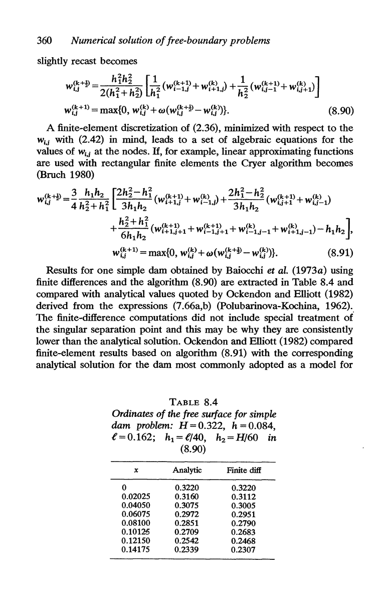
Results for

one

simple dam obtained by Baiocchi et

al.

(1973a) using

finite differences and the algorithm (8.90) are extracted in Table 8.4

and

compared with analytical values quoted by Ockendon and Elliott (1982)

derived from the expressions (7.66a,b) (Polubarinova-Kochina, 1962).

The

finite-difference computations did not include special treatment

of

the singular separation point and this may

be

why they are consistently

lower than the analytical solution. Ockendon and Elliott (1982) compared

finite-element results based on algorithm (8.91) with

the

corresponding

analytical solution for the dam most commonly adopted as a model for

TABLE

8.4

Ordinates

of

the

free

surface for simple

dam problem:

H = 0.322, h = 0.084,

f=0.162;

hI

=f/40,

h2

=H/60

in

(8.90)

x Analytic

Finite

di1f

0 0.3220

0.3220

0.02025

0.3160 0.3112

0.04050

0.3075

0.3005

0.06075

0.2972

0.2951

0.08100

0.2851 0.2790

0.1012!i

0.2709

0.2683

0.12150

0.2542

0.2468

0.14175

0.2339

0.2307

Variational inequality and complementarity methods

361

TABLE

8.S

Ordinates

of

the free surface for simple dam prob-

lem H = 1, h = 1/6, t

==

2/3

Finite element size

24x Analytic

1/24 1/48

0

1.0000

1.0000 1.0000

1

0.9894

0.9869 0.9885

2

0.9755 0.9735

0.9743

3

0.9593

0.9579 0.9586

4

0.9413 0.9378

0.9406

5 0.9215 0.9202 0.9207

6 0.8999 0.8966

0.8992

7

0.8765

0.8747 0.8757

8

0.8513 0.8496

0.8505

9 0.8240 0.8224 0.8235

10

0.7946

0.7934

0.7936

11

0.7628

0.7605 0.7607

12 0.7281 0.7256 0.7281

13 0.6900 0.6879

0.6900

14

0.6472 0.6467 0.6475

15

0.5975

0.6016 0.5932

16

0.5294 (separation point)

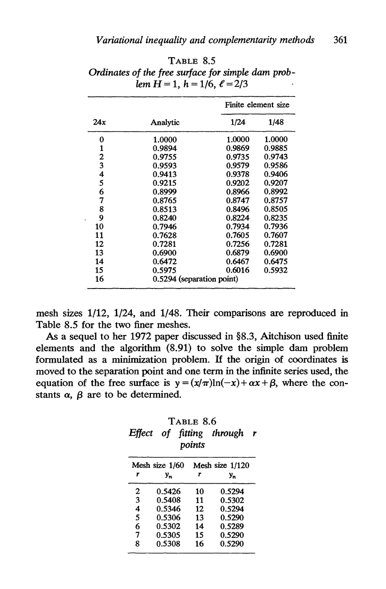
mesh sizes 1/12, 1/24,

and

1/48.

Their

comparisons

are

reproduced in

Table

8.S for

the

two finer meshes.

As

a sequel

to

her

1972

paper

discussed in §8.3, Aitchison used finite

elements

and

the

algorithm (8.91)

to

solve

the

simple

dam

problem

formulated as a minimization problem. H the origin

of

coordinates is

moved

to

the

separation point

and

one

term

in

the

infinite series used,

the

equation

of

the

free surface is y = (xhr )In(

-x)

+

ax

+

{3,

where

the

con-

stants a,

{3

are

to

be

determined.

TABLE

8.6

Effect

of

fitting

through

r

points

Mesh size 1/60 Mesh size 1/120

r

Y

n

r

Y

n

2

0.5426 10 0.5294

3 0.5408

11

0.5302

4

0.5346 12 0.5294

5

0.5306 13 0.5290

6

0.5302

14

0.5289

7

0.5305

15

0.5290

8 0.5308 16 0.5290

Crank J. Free and Moving Boundary Problems

Подождите немного. Документ загружается.