Devore J.L., Berk K.N. Modern Mathematical Statistics with Applications
Подождите немного. Документ загружается.


CHAPTER FOUR
Continuous
Random Variables
and Probability
Distributions
Introduction
As mentioned at the beginning of Chapter 3, the two important types of random
variables are discrete and continuous. In this chapter, we study the second general
type of random variable that arises in many applied problems. Sections 4.1 and 4.2
present the basic definitions and properties of continuous random variables, their
probability distributions, and their moment generating functions. In Section 4.3,
we study in detail the normal random variable and distribution, unquestionably the
most important and useful in probability and statistics. Sections 4.4 and 4.5 discuss
some other continuous distributions that are often used in applied work. In
Section 4.6, we introduce a method for assessing whether given sample data is
consistent with a specified distribution. Section 4.7 discusses methods for finding
the distribution of a transformed random variable.
J.L. Devore and K.N. Berk, Modern Mathematical Statistics with Applications, Springer Texts in Statistics,
DOI 10.1007/978-1-4614-0391-3_4,
#
Springer Science+Business Media, LLC 2012
158

4.1
Probability Density Functions
and Cumulative Distribution Functions
A discrete random variable (rv) is one whose possible values either constitute a
finite set or else can be listed in an infinite sequence (a list in which there is a first
element, a second element, etc.). A random variable whose set of possible values is
an entire interval of numbers is not discrete.
Recall from Chapter 3 that a random variable X is continuous if (1) possible
values comprise either a single interval on the number line (for some A < B, any
number x between A and B is a possible value) or a union of disjoint intervals, and
(2) P(X ¼ c) ¼ 0 for any number c that is a possibl e value of X.
Example 4.1 If in the study of the ecology of a lake, we make depth measurements at randomly
chosen locations, then X ¼ the depth at such a location is a continuous rv. Here A is
the minimum depth in the region being sample d, and B is the maximum depth.
■
Example 4.2 If a chemical compound is randomly selected and its pH X is determined, then X is a
continuous rv because any pH value between 0 and 14 is possible. If more is known
about the compound selected for analysis, then the set of possible values might be a
subinterval of [0, 14], such as 5.5 x 6.5, but X would still be continuous.
■
Example 4.3 Let X represent the amount o f time a randomly selected customer spends waiting
for a haircut before h is/her haircut commences. Your first thought might be that X is
a continuous random variable, since a measurement is required to determine its
value. However, there are customers lucky enough to have no wait whatsoever
before climbing into the barber’s chair. So it must be the case that P(X ¼ 0) > 0.
Conditional on no chairs being empty, though, the waiting time will be continuous
since X could then assume any value between some minimum possible time A and a
maximum po ssible time B. This random variable is neither purely discrete nor
purely continuo us but instead is a mixture of the two types.
■
One might argue that although in principle variables such as height, weight,
and temperature are continuous, in practice the limitations of our measuring
instruments restrict us to a discrete (though sometimes very finely subdivided)
world. However, continuous models often approximate real-world situations very
well, and continuous mathematics (the calculus) is frequently easier to work with
than the mathematics of discrete variables and distributions.
Probability Distributions for Continuous Variables
Suppose the variable X of interest is the depth of a lake at a randomly chosen point
on the surface. Let M ¼ the maximum depth (in meters), so that any number in the
interval [0, M] is a possible value of X. If we “discretize” X by measuring depth to
the nearest meter, then possible values are nonnegative integers less than or equal
to M. The resulting discrete distribution of depth can be pictur ed using a probability
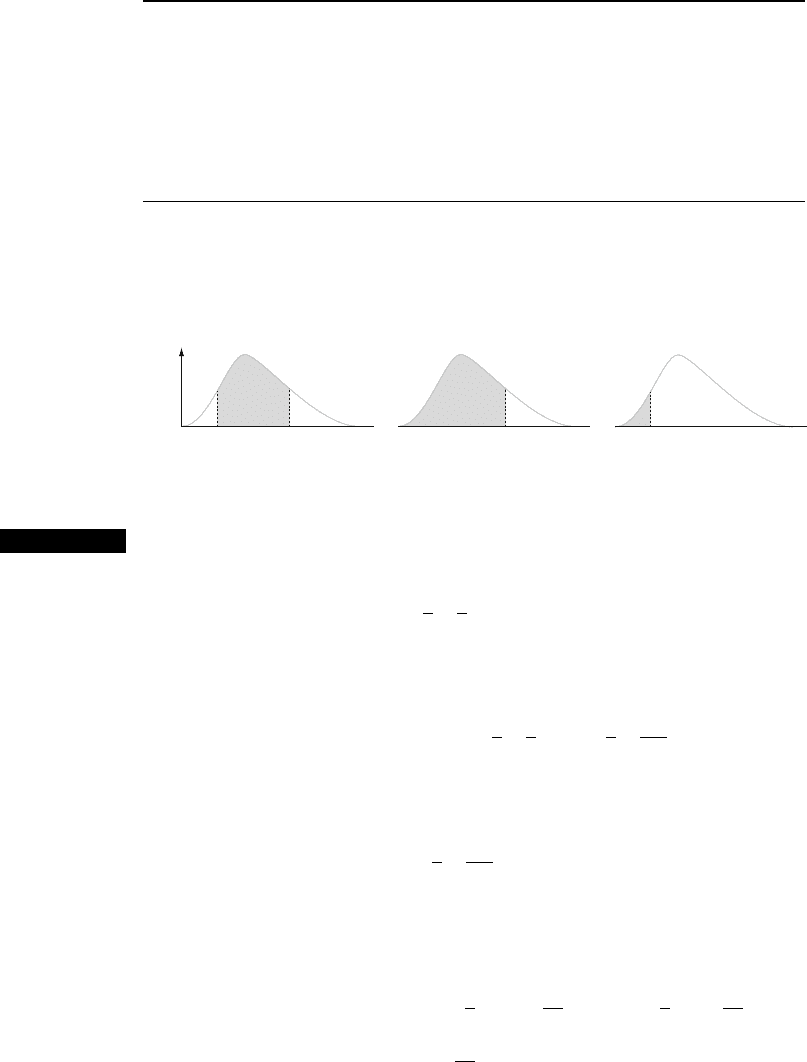
histogram. If we draw the histogram so that the area of the rectangle above any
possible integer k is the proportion of the lake whose depth is (to the nearest meter)
k, then the total area of all rectangles is 1. A possible histogram appears in
Figure 4.1(a).
4.1 Probability Density Functions and Cumulative Distribution Functions 159
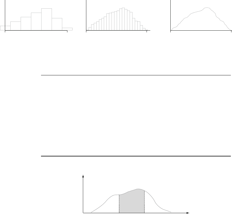
If depth is measured much more accurately and the same measurement axis
as in Figure 4.1(a) is used, each rectangle in the resulting probability histogram is
much narrower, although the total area of all rectangles is still 1. A possible
histogram is pictured in Figure 4.1(b); it has a muc h smoother appearance than
the histogram in Figure 4.1(a). If we continue in this way to measure depth more
and more finely, the resulting sequence of histograms approaches a smooth curve,
as pictured in Figure 4.1(c). Because for each histogram the total area of all
rectangles equals 1, the total area under the smooth curve is also 1. The probability
that the depth at a randomly chosen point is between a and b is just the area under
the smooth curve between a and b. It is exactly a smooth curve of the type pictured
in Figure 4.1(c) that specifies a continuous probability distribution.
DEFINITION
Let X be a continuous rv. Then a probability distribution or probability
density function (pdf) of X is a function f (x) such that for any two numbers a
and b with a b,
Pða X bÞ¼
ð
b
a
f ð xÞdx
That is, the probability that X takes on a value in the interval [a, b] is the area
above this interval and under the graph of the density function, as illustrated
in Figure 4.2. The graph of f(x) is often referred to as the density curve.
ab
x
f(x)
Figure 4.2
P
(
a
X
b
) ¼ the area under the density curve between a and b
ab c
0
M
0
M
0
M
Figure 4.1 (a) Probability histogram of depth measured to the nearest meter; (b) probability histogram
of depth measured to the nearest centimeter; (c) a limit of a sequence of discrete histograms
160
CHAPTER 4 Continuous Random Variables and Probability Distributions
For f(x) to be a legitimate pdf, it must satisfy the following two conditions:
1. f(x) 0 for all x
2.
Ð
1
1
f ð xÞdx ¼ area under the entire graph of f ðxÞ½¼1
Example 4.4 Th e direction of an imperfection with respect to a reference line on a circular object
such as a tire, brake rotor, or flywheel is, in general, subject to uncertainty.
Consider the reference line connecting the valve stem on a tire to the center
point, and let X be the angle measured clockw ise to the location of an imperfection.
One possible pdf for X is
f ð xÞ¼
1
360
0 x <360
0 otherwise
8
<
:
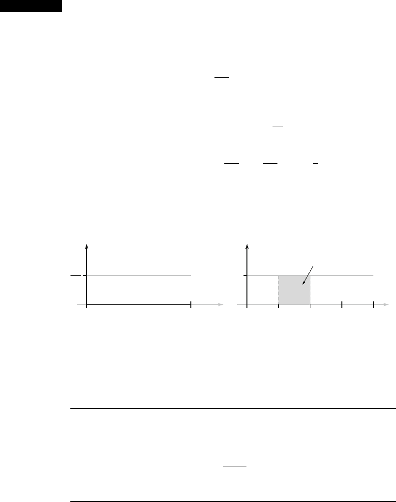
The pdf is graphed in Figure 4.3. Clearly f(x) 0. The area under the density curve
is just the area of a rectangle: ðheightÞðbaseÞ¼
1
360
ð360Þ¼1. The probability
that the angle is between 90
and 180
is
Pð90 X 180Þ¼
ð
180
90
1
360
dx ¼
x
360
x¼180
x¼90
¼
1
4
¼ :25
The probability that the angle of occurrence is within 90
of the reference line is
Pð0 X 90ÞþPð270 X<360Þ¼:25 þ :25 ¼ :50
Because whenever 0 a b 360 in Example 4.4, P(a X b) depends only
on the width b a of the interval, X is said to have a uniform distribution.
DEFINITION
A continuous rv X is said to have a uniform distribution on the interval [A, B]
if the pdf of X is
f ð x; A; BÞ¼
1
B A
A X B
0 otherwise
8
<
:
x
1
360
0 360
x
36027018090
f(x) f(x)
Shaded area = P(90 ≤ X ≤ 180)
Figure 4.3 The pdf and probability for Example 4.4 ■
4.1 Probability Density Functions and Cumulative Distribution Functions 161

The graph of any uniform pdf looks like the graph in Figure 4.3 except that the
interval of positive density is [A, B] rather than [0, 360].
In the discrete case, a probability mass functi on (pmf) tells us how little
“blobs” of probability mass of various magnitudes are distributed along the mea-
surement axis. In the continuous case, probability densi ty is “smeared” in a
continuous fashion along the interval of possible values. When density is sme ared
uniformly over the interv al, a uniform pdf, as in Figure 4.3, results.
When X is a discrete random variable, each possible value is assigned
positive probability. This is not true of a continuous random variable (that is,
the second condition of the definition is satisfied) because the area under a density
curve that lies above any single value is zero:
PðX ¼ cÞ¼
ð
c
c
f ð xÞdx ¼ lim
e ! 0
ð
cþe
ce
f ð xÞdx ¼ 0
The fact that P(X ¼ c) ¼ 0 when X is continuo us has an im portant practical
consequence: The probability that X lies in some interval between a and b does not
depend on whether the lower limit a or the upper limit b is included in the
probability calculation:
Pða X bÞ¼Pða < X < bÞ¼Pða < X bÞ¼Pða X < bÞð4: 1 Þ
If X is discrete and both a and b are possibl e values (e.g., X is binomial with n ¼ 20
and a ¼ 5, b ¼ 10), then all four of these probabilities are different.
The zero probability condition has a physical analog. Consider a solid
circular rod with cross-sectional area ¼ 1in
2
. Place the rod alongside a measure-
ment axis and suppose that the density of the rod at any point x is given by the value
f(x) of a density function. Then if the rod is sliced at points a and b and this segment
is removed, the amount of mass removed is
Ð
b
a
f ðxÞdx; if the rod is sliced just at the
point c, no mass is removed. Mass is assigned to interval segments of the rod but
not to individual points.
Example 4.5 “Time headway” in traffic flow is the elapsed time between the time that one car
finishes passing a fixed point and the instant that the next car begins to pass that point.
Let X ¼ the time headway for two randomly chosen consecutive cars on a freeway
during a period of heavy flow. The following pdf of X is essentially the one suggested
in “The Statistical Properties of Freeway Traffic” (Transp. Res., 11: 221–228):
f ðxÞ¼
:15e
:15ðx:5Þ
x :5
0 otherwise
The graph of f(x) is given in Figure 4.4; there is no density associated with
headway times less than .5, and headway density decreases rapidly (exponentially
fast) as x increases from .5. Clearly, f(x) 0; to show that
Ð
1
1
f ð xÞdx ¼ 1 we use
the calculus result
Ð
1
a
e
kx
dx ¼ 1=kðÞe
ka
. Then
ð
1
1
f ðxÞdx ¼
ð
1
:5
:15e
:15ðx:5Þ
dx ¼ :15e
:075
ð
1
:5
e
:15x
dx
¼ :15e
:075
1
:15
e
:15ð:5Þ
¼ 1
162 CHAPTER 4 Continuous Random Variables and Probability Distributions
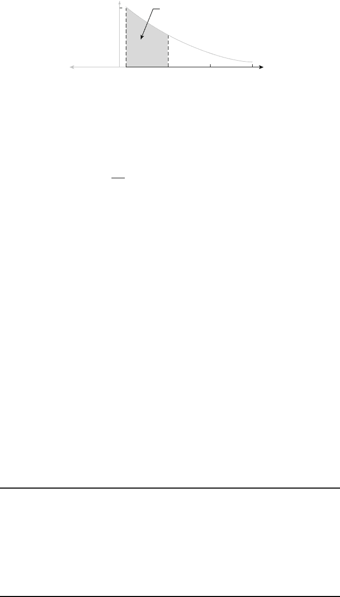
The probability that headway time is at most 5 s is
PðX 5Þ¼
ð
5
1
f ð xÞdx ¼
ð
5
:5
:15e
:15ðx:5Þ
dx ¼ :15e
:075
ð
5
:5
e
:15x
dx
¼ :15e
:075
1
:15
e
:15x
x¼5
x¼:5
¼ e
:075
ðe
:75
þ e
:075
Þ
¼ 1:078ð:472 þ :928Þ¼:491 ¼ Pðless than 5 sÞ¼PðX<5Þ
■
Unlike discrete distributions such as the binomial, hypergeometric, and
negative binomial, the distribution of any given continuous rv cannot usually be
derived using simpl e probabilistic arguments. Instead, one must make a judicious
choice of pdf based on prior knowledge and available data. Fortunately, some
general pdf families have been found to fit well in a wide variety of experimental
situations; several of these are discussed later in the chapter.
Just as in the discrete case, it is often helpful to think of the population of
interest as consisting of X values rather than individuals or objects. The pdf is then a
model for the distribution of values in this numerical population, and from this
model various population characteristics (such as the mean) can be calculated.
Several of the most important concepts introduced in the study of discrete
distributions also play an important role for continuous distributions. Definitions
analogous to those in Chapter 3 involve replacing summation by integration.
The Cumulative Distribution Function
The cumulative distribution function (cdf) F(x) for a discrete rv X gives, for
any specified number x, the probability P(X x). It is obtained by summing the
pmf p( y) over all possible values y satisfying y x. The cdf of a continuous rv
gives the same probabilities P(X x) and is obtained by integrating the pdf f(y)
between the limits 1 and x.
DEFINITION
The cumulative distribution function F(x) for a continuous rv X is defined
for every number x by
FðxÞ¼PðX xÞ¼
ð
x
1
f ð yÞdy
For each x, F(x) is the area under the density curve to the left of x. This is
illustrated in Figure 4.5, where F(x ) increases smoothly as x increases.
x
.15
.5 5 10 15
f (x)
P
(X
≤ 5)
0
Figure 4.4 The density curve for headway time in Example 4.5
4.1 Probability Density Functions and Cumulative Distribution Functions 163
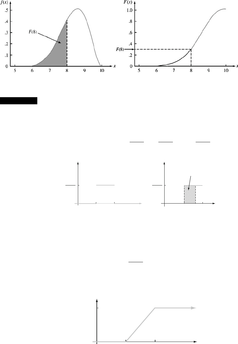
Example 4.6 Let X, the thickness of a membrane, have a uniform distribution on [A, B]. The
density function is shown in Figure 4.6. For x < A, F(x) ¼ 0, since there is no area
under the graph of the density function to the left of such an x. For x B, F(x) ¼ 1,
since all the area is accumulated to the left of such an x. Finally, for A x B,
FðxÞ¼
ð
x
1
f ð yÞdy ¼
ð
x
A
1
B A
dy ¼
1
B A
y
y¼x
y¼A
¼
x A
B A
The entire cdf is
FðxÞ¼
0 x < A
x A
B A
A x < B
1 x B
8
>
>
<
>
>
:
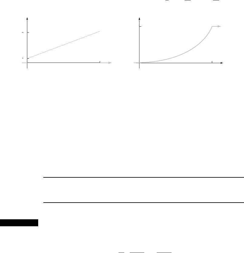
The graph of this cdf appears in Figure 4.7.
1
AB
AB
x
x
f(x )
B
− A
1
B − A
Shaded area = F (x)
Figure 4.6 The pdf for a uniform distribution
AB
x
1
F(x)
Figure 4.7 The cdf for a uniform distribution ■
Figure 4.5 A pdf and associated cdf
164
CHAPTER 4 Continuous Random Variables and Probability Distributions
Using F(x) to Compute Probabilities
The import ance of the cdf here, just as for discrete rv’s, is that probabilities of
various intervals can be computed from a formula or table for F(x).
PROPOSITION
Let X be a continuous rv with pdf f(x) and cdf F(x). Then for any number a ,
PX> aðÞ¼1 FðaÞ
and for any two numbers a and b with a < b,
Pa X bðÞ¼FðbÞFðaÞ
Figure 4.8 illustrates the second part of this proposition; the desired probability is
the shaded area under the density curve between a and b, and it equals the
difference between the two shaded cumulative areas.
Example 4.7 Sup pose the pdf of the magnitude X of a dynamic load on a bridge (in newtons) is
given by
f ð xÞ¼
1
8
þ
3
8
x 0 x 2
0 otherwise
8
<
:
For any number x between 0 and 2,
FðxÞ¼
ð
x
1
f ðyÞdy ¼
ð
x
0
1
8
þ
3
8
y
dy ¼
x
8
þ
3x
2
16
Thus
FðxÞ¼
0 x < 0
x
8
þ
3x
2
16
0 x 2
12< x
8
>
>
<
>
>
:
The graphs of f(x) and F(x) are shown in Figure 4.9. The probability that the load is
between 1 and 1.5 is
Pð1 X 1:5Þ¼Fð1:5ÞFð1Þ¼
1
8
ð1:5Þþ
3
16
ð1:5Þ
2
1
8
ð1Þþ
3
16
ð1Þ
2
¼
19
64
¼ :297
ab b a
f(x)
=
−
Figure 4.8 Computing P(a X b) from cumulative probabilities
4.1 Probability Density Functions and Cumulative Distribution Functions 165
The probability that the load exceeds 1 is
PðX > 1Þ¼1 PðX 1Þ¼1 Fð1Þ¼1
1
8
ð1Þþ
3
16
ð1Þ
2
¼
11
16
¼ :688
■
Once the cdf has been obtained , any probability involving X can easily be
calculated without any further integration.
Obtaining f(x) from F(x)
For X discrete, the pmf is obta ined from the cdf by taking the difference between
two F(x) values. The continuous analog of a difference is a derivative. The
following result is a consequence of the Fundamental Theorem of Calculus.
PROPOSITION
If X is a continuous rv with pdf f(x) and cdf F(x), then at every x at which the
derivative F
0
(x) exists, F
0
(x) ¼ f(x).
Example 4.8
(Example 4.6
continued)
When X has a uniform distribution, F(x) is differentiable except at x ¼ A and
x ¼ B, where the graph of F(x) has sharp corners. Since F(x) ¼ 0 for x < A
and F(x) ¼ 1 for x > B, F
0
(x) ¼ 0 ¼ f(x) for such x. For A < x < B,
F
0
ðxÞ¼
d
dx
x A
B A
¼
1
B A
¼ f ðxÞ
■
Percentiles of a Continuous Distribution
When we say that an individual’s test score was at the 85th percentile of the
population, we mean that 85% of all population scores were below that score and
15% were above. Similarly, the 40th percentile is the score that exceeds 40% of all
scores and is exceeded by 60% of all scores.
1
8
7
8
20
2
1
x
x
f(x)
F(x)
Figure 4.9 The pdf and cdf for Example 4.7
166
CHAPTER 4 Continuous Random Variables and Probability Distributions
DEFINITION
Let p be a number between 0 and 1. The (100p)th percentile of the distribu-
tion of a continuous rv X, denoted by (p), is defined by
p ¼ F½ðpÞ ¼
ð
ðpÞ
1
f ð yÞdy ð4:2Þ
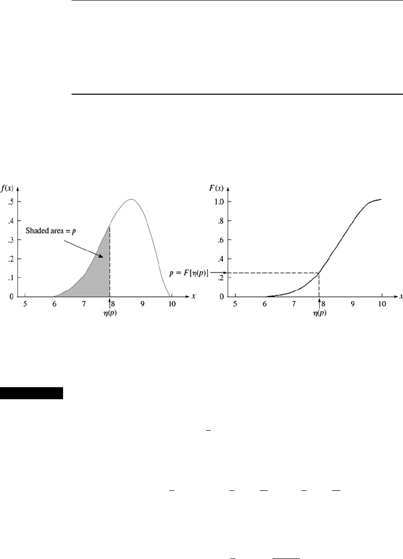
According to Expression (4.2), (p) is that value on the measurement axis such that
100p% of the area under the graph of f(x) lies to the left of (p) and 100(1 p)%
lies to the right. Thus (.75), the 75th percentile, is such that the area under the
graph of f(x) to the left of (.75) is .75. Figure 4.10 illustrates the definition.
Example 4.9 Th e distribution of the amount of gravel (in tons) sold by a construction supply
company in a given week is a continuous rv X with pdf
f ð xÞ¼
3
2
ð1 x
2
Þ 0 x 1
0 otherwise
(
The cdf of sales for any x between 0 and 1 is
FðxÞ¼
ð
x
0
3
2
ð1 y
2
Þdy ¼
3
2
y
y
3
3
y¼x
y¼0
¼
3
2
x
x
3
3
The graphs of both f(x) and F(x) appear in Figure 4.11. The (100p)th percentile of
this distribution satisfies the equation
p ¼ F½ðpÞ ¼
3
2
ðpÞ
ðpÞ½
3
3
"#
Figure 4.10 The (100p)th percentile of a continuous distribution
4.1 Probability Density Functions and Cumulative Distribution Functions 167