Dorst L., Fontijne D., Mann S. Geometric Algebra for Computer Science. An Object Oriented Approach to Geometry

Подождите немного. Документ загружается.

442 CONSTRUCTIONS IN EUCLIDEAN GEOMETRY CHAPTER 15

(a) (b) (c)

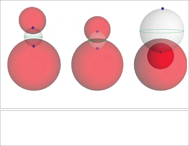
Figure 15.3: The meet and plunge of two spheres at increasing distances. When they do

not intersect (a,c), the red dual spheres have a real

plunge and an imaginary meet. When

they do intersect (b), the

meet is real and the plunge imaginary. In all cases meet and

plunge are each other’s dual (i.e., polars on the three white spheres). Imaginary elements

are depicted as speckled.

15.1.4 THE PLUNGE OF FLATS

The construction of a general ﬂat p ∧ E ∧∞can also be interpreted as a plunge.Asa

deﬁnite example, let us interpret the line p∧u∧∞. According to the

plunge construction,

this should perpendicularly intersect the points p and ∞ (so that it contains them), and

it should moreover be perpendicular to u

∗

, which is the plane through the origin with

normal vector u. Obviously, this

plunge must then be the direct representation of the

line through p in the u direction. This is illustrated in Figure 15.4(a). Including another

Euclidean vector factor v gives an element that should meet the dual line u ∧ v perpen-

dicularly, and is therefore the direct representation of a plane. Removing the Euclidean

factor (by setting it equal to the 0-blade 1) gives the representation of a ﬂat of dimension

zero (i.e., a direct ﬂat point p ∧∞, which is the element that perpendicularly connects the

small dual sphere p with the point at inﬁnity ∞).

Now let us revisit the object p(c ∧∞) from (14.4), which contains such a ﬂat point in

its construction. It was a dual sphere through the point p, with center c. Undualizing this,

we ﬁnd that it is the direct object

S = p ∧ (c ∧∞)

−∗

SECTION 15.1 EUCLIDEAN INCIDENCE AND COINCIDENCE 443

(a) (b)

Figure 15.4: (a) The plunge construction of the line p ∧ u ∧∞. (b) Visualization of the point

c ∧∞and its consistency with constructing the dual sphere p(c ∧∞), given a point p.

We see that this indeed contains p (it plunges into p since it is a direct representation of

the form p∧), and that we should think of it as also plunging into the ﬂat point c ∧∞.We

have just seen that such a ﬂat point in itself is the

plunge of c and ∞, connecting those two

dual elements. We observe that we get an intuitively satisfying picture like Figure 15.4(b),

in which the ﬂat point c ∧∞has “hairs” extending from c to inﬁnity. Intersecting all of

those perpendicularly while also passing through the given point p must produce a sphere.

Carrying this type of thinking to its logical extreme, we can also interpret a purely

Euclidean blade such as v ∧ u as a direct element of our geometry. Since it is a purely

Euclidean 2-blade, we have already met it as the dual representation of the line that is the

meet of the two dual planes u and v passing through the origin. But if we interpret v ∧ u

directly, it should be the

plunge of the two planes represented dually by u and v (i.e., the

general element that is perpendicular to both).

Any cylinder with their common line as its axis is a solution, so this is like a nest of cylin-

ders of arbitrary radius but ﬁxed axis. However, as soon as we try to pick out one of the

cylinders by specifying a point p on it, the element p ∧ (v ∧u) is a unique circle.Soamore

accurate description is that v ∧ u represents a stack of nests of circles. But that is also not

quite right, since these elements are not circles yet (we have speciﬁed only a grade 2 object,

not grade 3); rather, v ∧ u is a stack of nests of potential circles. This may seem like an

uncommon object, until you realize that a rotation rotor can be made from this dual line

∗

= v ∧ u as exp(α v ∧ u). Then the element L

∗

= v ∧ u in fact describes a collection of

444 CONSTRUCTIONS IN EUCLIDEAN GEOMETRY CHAPTER 15

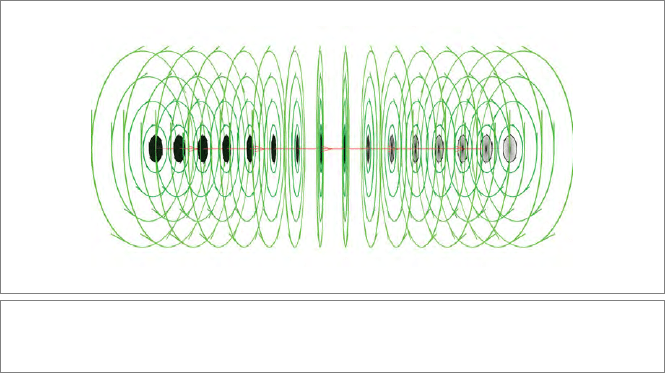
Figure 15.5: The circular orbits of a line L, which are p ∧ L

∗

for various points p. The orbits

of points on the line are tangent bivectors, depicted as small oriented disks.

orbits of the rotating points, as indicated in Figure 15.5 (in which the actual orbits p ∧ L

∗

are drawn).

The point of all this discussion is that the conformal model suggests, in its algebraic coher-

ence, a consistent and rich language for Euclidean geometry. It contains objects that we

have not seen this explicitly before, but that on closer scrutiny represent familiar geomet-

ric concepts, and endows them with precise computational properties. Now that we have

an algebraic way to combine them, it pays to try and get them into more practical form

into our intuition, so that we can use them as active concepts in the solution of problems.

This takes practice, and we recommend playing with interactive software packages like

GAViewer to absorb this into your intuition—the old-fashioned derivations on paper are

rather useless for this (though they should be used to check and/or prove the correctness

of your new insights).

15.2 EUCLIDEAN NUGGETS

When you work with the conformal model in a practical application, you will ﬁnd that you

often need to convert elements, and that certain operations appear to be useful nuggets,

occurring again and again. We provide some in this section, and try to discern some pat-

terns. This is certainly not a complete inventory of such elementary constructions. We

hope that the techniques we expose in deriving them will give you the skills to derive your

own special expressions, should your application require them.

SECTION 15.2 EUCLIDEAN NUGGETS 445

15.2.1 TANGENTS WITHOUT DIFFERENTIATING

When you need the tangent to a ﬂat Π or to a round Σ passing through one of its points p,

you can compute this without differentiation. Calling the element X (so that p ∧ X = 0),

its tangent is

tangent to X at p: p



(15.1)

The tangents are illustrated in Figure 15.6.

The formula is easy to prove for a ﬂat through the origin: o(o ∧ E ∧∞)= o ∧ E, and

because of Euclidean covariance, this holds everywhere for any ﬂat. For a round the proof

is also most simply done at the origin o. A direct round through o with center c and direc-

tion E ∞is o∧



c(−



E ∞)



, according to structural exercise 4. Then the proposed formula

(15.1) gives, by straightforward computation, that the tangent equals o ∧ (cE),whichis

the correct result in its geometrical aspects: its directional part is an element of the carrier

E, perpendicular to the radial vector. Note that this local tangent blade is weighted by the

magnitude of the radial vector c, which is the radius ρ. The occurrence of ρ (rather than

) may seem to require complex numbers for imaginary rounds. However, imaginary

rounds contain no real points, so they have no real tangents either.

15.2.2 CARRIERS, TANGENT FLAT

Let us deﬁne the carrier of an element as the smallest grade ﬂat that contains it. A ﬂat is

therefore its own carrier. The carrier of a round Σ (which may be a tangent) is

carr ier of round Σ: Σ ∧∞.

This is easily proved:



(c +

∞) ∧ E



∧∞= c ∧ E ∧∞.

We can use this to compute the tangent ﬂat to an element X at one of its points p as

(p



X ) ∧∞. This applies to rounds and ﬂats alike; though for a ﬂat it is the identity.

Tangents do not have tangent ﬂats, though they do have a carrier.

p ⎦ K

∧

⎦ Λ

∧

p ⎦ ∑

∧

p ⎦ ∏

∧

Figure 15.6: The tangents of ﬂats and rounds at one of their points are simply computed

by the contraction. No differentiation is required.

446 CONSTRUCTIONS IN EUCLIDEAN GEOMETRY CHAPTER 15

15.2.3 SURROUNDS, FACTORIZATION OF ROUNDS

A round Σ can be surrounded by the smallest sphere containing it. In its dual

representation, that surround of Σ is

surround of round Σ:

Σ ∧∞

, (15.2)

in which the division denotes right division (i.e., Σ (Σ ∧∞)

−1

). This even applies to

tangents, but it then returns the locational point of the tangent, in agreement with the

intuition that a tangent has zero size. Formula (15.2) can be interpreted as the dual of Σ

relative to the carrier of dimension k; therefore the expression equals (c −

∞)(−1)

which is a dual sphere containing Σ. We prove the surround formula below.

If the round Σ is given in its dual form, you need the dual of (15.2):

surround of dual round σ: (−1)

σ

∞σ

. (15.3)

The signs ensure that the computed surround is the same as before, but you could ignore

them.

A round can be factored as the geometric product of its surround and its carrier:

factorization of a round Σ: Σ=



Σ ∧∞



(Σ ∧∞), (15.4)

and its dual is

factorization of a dual round σ: σ =



∞σ



(∞σ), (15.5)

in which you need to include the (−1)

(as in (15.3)) if you need the proper orienta-

tion of the surround. These unique factorization formulas are the motivation behind the

expression for the surrounding sphere. It is easy to show that the center of the surround-

ing sphere is in the carrier plane; and then (15.4) actually represents the perpendicular

meet of carrier and surround. This makes the factorization geometrically very natural

(see Figure 15.7). Algebraically, this factorization in orthogonal factors is important in

symbolic simpliﬁcation of formulas involving rounds. Given a round like a circle, such

a factorization gives us a better understanding of it: the carrier plane gives us direction,

weight, and orientation of the circle, and the sphere gives us its location (i.e., center) and

size (i.e., radius squared).

A special case is a point pair, for which the same formulas hold, for it is clearly also a round.

Now Σ ∧∞represents the carrier line, and division again gives the containing sphere, as

shown in Figure 15.7. The result is an expression for the smallest sphere containing two

points:

p ∧ q

p ∧ q ∧∞

(p ∧ q)(p ∧ q ∧∞)

−2p · q

= −



p + q + (p · q)∞



SECTION 15.2 EUCLIDEAN NUGGETS 447

Figure 15.7: The factorization of rounds, using their carrier and surround. A point pair P is

factorized as the intersection of its surrounding dual sphere P/(P ∧∞) and the carrier line P∧∞.

A circle K is factorized as the intersection of the dual surrounding sphere K/(K ∧∞) and the

carrier plane K ∧∞.

The overall sign in this makes the meet correct, but you can ignore it if you are not inter-

ested in such matters of orientation.

For the proof of the correctness of the surround formula (15.2), we need to show that the

center of the surround is in the carrier plane. So we reﬂect the surround in that plane and

verify that this merely changes the surround by a sign. Using the reﬂection formula for a

dual element into a directly represented mirror (from Table 7.1), we ﬁnd that the deriva-

tion is quicker when we reﬂect in the inverse of the carrier (which makes no difference

geometrically). We obtain

(Σ ∧∞)

−1



Σ (Σ ∧∞)

−1



(Σ ∧∞) = (Σ ∧∞)

−1

Σ=



Σ (Σ ∧∞)

−1

so that this dual sphere becomes a signed multiple of itself (in the ﬁnal transition, we took

the reverse and computed the resulting sign, after realizing that the reverse of a vector is

the vector itself). It follows that the center of the sphere is on the mirroring carrier. As a

consequence, the outer product of the dual surround sphere with the carrier must be zero;

therefore you can replace the geometric product in (15.4) with a contraction, showing

clearly that it expresses a

meet of the carrier with the surround (in that order).

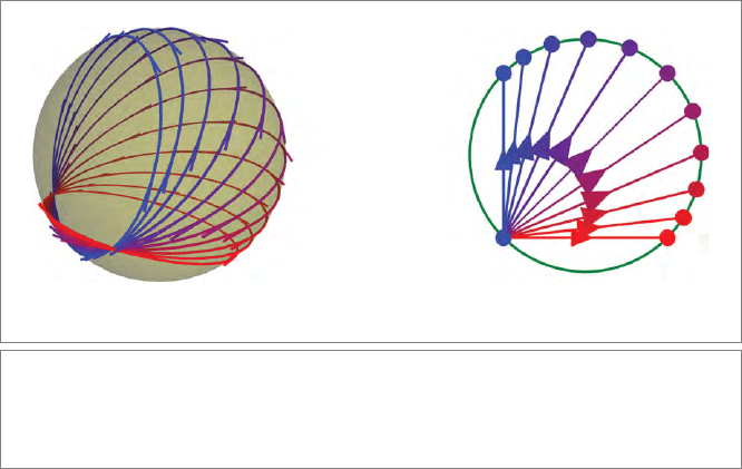
15.2.4 AFFINE COMBINATIONS

An afﬁne combination of two normalized points gives a 1-parameter family of normalized

dual spheres (so not of points!):

λ p + (1 − λ) q.

(15.6)

The corresponding dual spheres are depicted in Figure 15.8 for the 2-D case. As λ becomes

inﬁnite, the dual sphere approaches the midplace p − q (with enormous weight).

448 CONSTRUCTIONS IN EUCLIDEAN GEOMETRY CHAPTER 15

These dual spheres all intersect the smallest dual sphere through p and q orthogonally, as

you may easily verify:



λ p + (1 − λ) q





(p + q) +

(p · q) ∞



= 0.

Their radius squared is −λ(1 − λ) d

(p, q ), so that imaginary dual spheres result for 0 <

λ < 1. (Those imaginary dual spheres do not look orthogonal to the smallest containing

sphere in Figure 15.8, but their inner product with it is indeed zero.) Comparing this

to the treatment in the homogeneous model where this afﬁne combination is used in

Section 11.2.3 to obtain the points between p and q, we ﬁnd that the centers of the resulting

dual spheres certainly behave exactly like the locations in the afﬁne interpolation, though

they are surrounded by imaginary dual spheres for the values of interest. To mimic that

interpolation precisely within the conformal model, you should interpolate ﬂat points

rather than zero-radius dual spheres: λ (p ∧∞) + (1 − λ)(q ∧∞) is the ﬂat point at

location λ p + (1 − λ) q.

Within the conformal model, other afﬁne combinations become feasible. The afﬁne com-

binations of ﬂats are a simple extension of those seen in the homogeneous model in

Section 11.2.3 and require little explanation. As there, 3-D lines can only be added if they

have a ﬁnite point in common, which implies in the conformal model that they have

two points in common, one of which is the point at inﬁnity. Two circles K

and K

can

now also be afﬁnely combined, but like lines only if they have a point pair in common

(which may be imaginary, as it usually is for two circles in a common plane); their sum

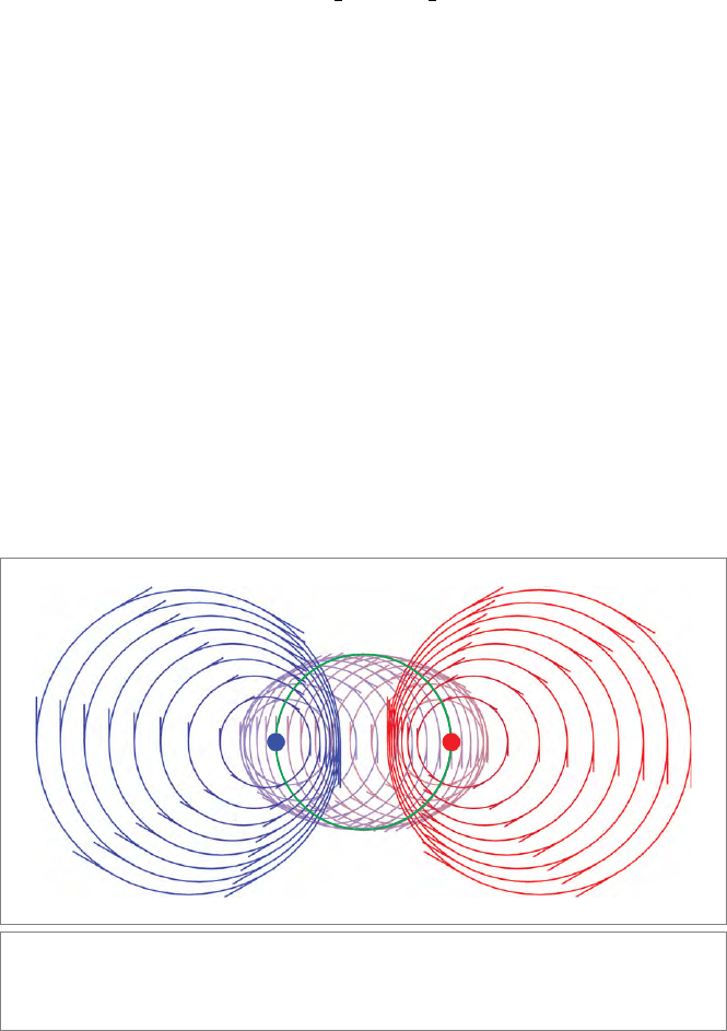
Figure15.8: Afﬁne combinations of the point p (red) and q (blue) in the plane are dual circles.

The amount of each point is indicated by the color mixture. Imaginary circles result for some

values; they have been dashed, and their centers follow the regular afﬁne interpolation.

SECTION 15.3 EUCLIDEAN PROJECTIONS 449

(a) (b)

Figure 15.9: Afﬁne combination of circles (a) and point pairs (b). These only generate other

objects if they form a 1-parameter family, which implies that they should have a point pair or

point in common, respectively. We show equal increments of the afﬁne parameter to demon-

strate its nonlinear relationship to angles or arcs.

then sweeps out circles on the common sphere K

∪ K

also containing the point pair, as

illustrated in Figure 15.9(a). Similarly, two point pairs can be combined afﬁnely if they

have one point in common, and the results are point pairs that sweep out the circle that

is their

join, illustrated in Figure 15.9(b).

All these additive combinations transform covariantly, so they are geometrically sensible

constructions. But you should avoid using them, for they parameterize the intermediate

elements awkwardly. It is much more preferable to use the two generative elements to

produce a rotor that affects the transformations; its parameters can be directly interpreted

as angles and scalings of the intermediate elements. We develop that technique in the next

chapter.

15.3 EUCLIDEAN PROJECTIONS

In geometric algebra, the projection of a blade X onto a blade P is another blade:

X → (XP)/P, (15.7)

where the division uses the geometric product. Applying this to the conformal model, we

ﬁnd the expected projection behavior if X is a ﬂat (as we will show below when discussing

Figure 15.10(b)).

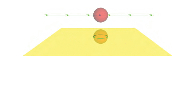
But when X is a round, this is not the projection you might expect. For instance, consider

Figure 15.10(a), the projection of a circle onto a plane. You may have hoped for an ellipse,

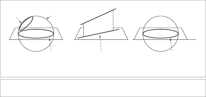
450 CONSTRUCTIONS IN EUCLIDEAN GEOMETRY CHAPTER 15

but an ellipse is not represented by a blade in our model, and therefore cannot be the

outcome of (15.7). Instead, the result of the projection of a circle onto a plane is a partic-

ular circle. To explain this effect, and derive precisely which circle, we recall (11.17):

A ∩ (X ∧ A

−∗

) = (X ∧ A

−∗

)

∗

A = (XA)A.

So the projection is proportional to the

meet of A with X ∧ A

−∗

(by the magnitude A

−2

In our Euclidean situation, the latter is the

plunge of X into A: it contains X and inter-

sects A perpendicularly. In the case of projecting a circle onto a plane, we indeed get the

construction of Figure 15.10(a), resulting in a circle that is the equator of the sphere that

plunges into the plane and contains the circle C.

It is instructive to see what happens for ﬂats, for instance when X is a line L and A a plane

Π as in Figure 15.10(b). Now L ∧ Π

∗

is the plane containing L perpendicular to Π, which

is itself a ﬂat. Therefore the

meet with Π now produces the expected line onto the plane

that is the orthogonal projection of the line onto the plane in the usual sense.

Figure 15.10(c) shows that when X is a line L and A is a sphere S,wegetagreatcircleon

the sphere, which is indeed a sensible interpretation of what it would be to project a line

on a sphere. Obviously, these examples generalize to the other elements we have treated.

You can even project a tangent vector onto a sphere (and the result is the point pair in

which the plunging circle containing the tangent vector meets the sphere).

In summary, the operation of projection generalizes from ﬂats in a sensible, but somewhat

unusual manner, providing a fundamental operation that seems to be new to Euclidean

geometry. We have yet to discover applications in which it might be useful to encode these

constructions compactly.

(a) (b) (c)

⎦ )/

⎦ S)/S

C∧

∏

∗

L∧

∏

∗

L∧S

∗

∏

∏ ∏

∏∏

Figure 15.10: Orthogonal projections in the conformal model of Euclidean geometry.

SECTION 15.4 APPLICATION: ALL KINDS OF VECTORS 451

15.4 APPLICATION: ALL KINDS OF VECTORS

In the classical way of computing with geometry, we have different needs for indicating

1-D directional aspects. They all use a vector u, but in different ways, which should trans-

form in different manners to be consistent with that usage.

We may just mean the direction u in general, which is a free vector that can occur at any

location. Or we may attach a vector to a point p to make a tangent vector p at the location

u (which feels more like two geometrical elements put together rather than as a uniﬁed

concept). In 3-D, a normal vector can be used to denote a plane; it can be placed anywhere

in that plane (this practice generalizes to hyperplanes in n-D). The direction vector of a

line gives it an afﬁne length measure that can be used anywhere along it; such a vector

is free to slide along the line. Finally, a position vector is used to denote the location of a

point relative to another point (the origin). This is actually a tangent vector that is always

attached to the origin (though in coordinate-based approaches, the origin is often left

implicitly understood).

Each of these concepts can be deﬁned as an element in the conformal model, and

this makes them have precisely the right transformation properties. Of course this is

true for higher-dimensional directional elements as well, and we have treated them

all above. But it pays to treat the vectors separately and explicitly. You know them

intimately, and may have come across problems in modeling and coding in which

the coordinate approach just was not speciﬁc enough to specify permitted transfor-

mations. The typical solution would be to deﬁne different data structures for each,

with their own methods [24, 13]. The conformal model offers an alternative: use pre-

cise algebraic elements that have the correct transformational properties, and then use

just general methods (versors) to transform them. Each object automatically trans-

forms correctly. Moreover, its clear algebraic relationship to the other computational

elements dispenses with the need for a profusion of new methods explicitly specifying

the various interactions. The algebraic data structures automatically perform compu-

tation and administration at the same time.

So, let us make these types of vectors; they are illustrated in Figure 15.11.

•

Free Vector u ∧∞. A 1-D direction without location is represented by the element

u ∧∞= u ∞. Its directional aspect is exhibited by applying a rotation rotor to it:

R[u ∧∞] = R[u] ∧ R[∞] = R[u] ∧∞,

which shows that u is the element denoting its direction. Applying a translation

rotor gives

[u ∧∞] = T

[u] ∧ T

[∞] =



u + (p · u) ∞



∧∞= u ∧∞,