Gao R.X., Yan R. Wavelets: Theory and Applications for Manufacturing

Подождите немного. Документ загружается.

ði; jÞ¼

i; f

 m

j; f

i; f

þ s

j; f

(8.12)

The symbols m

i; f

, m

j; f

and s

i; f

, s

j; f

represent the mean values and the variances of

the lth feature, f

, and for the classes i and j, respective ly. Since typically more than

two defect severity levels need to be evaluated in a machine defect diagnosis

system, a k-class, p feature component problem with kðk  1Þ=2 class pairs is

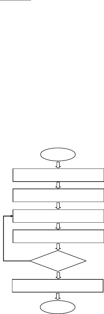
investigated for generality. The process for feature selection, based on the FLD

analysis method, is illustrated in Fig. 8.3.

Features (i.e., subband energy and kurtosis values) are ﬁrst extracted by

means of the WPT from the signals measured on the machine (e.g., a milling

machine, a spindle), under various operating conditions (e.g., speed and load).

The mean values and variances of each individual feature f

corresponding

to each machine status are then calculated, for each set of operation conditions

(e.g., 1,200 rpm, 3.6 kN radial load). For each possible class pair

fði; jÞji ¼ 1; 2; ...; k  1; j ¼ i þ 1; i þ 2; ...; k

formed from two different

machine states (e.g., health vs. light defect), the discriminant power measure J

ði; jÞ

for each feature f

, is calculated, using (8.12). Descending sorting J

ði; jÞ yields:

Start

End

Sub-band feature f

extraction

Condition pair (i,j) selection

Discriminant power J

(i,j) calculation

Feature subset F

i,j

selection

Final feature set F

final

selection

Next class

pair exist ?

Fig. 8.3 Flowchart of the

FLD feature selection process

130 8 Wavelet Packet Transform for Defect Severity Classiﬁcation

ði; jÞJ

ði; jÞJ

ði; jÞ (8.13)

The ﬁrst group of d features that have the highest relative J

ði; jÞ values are chosen

to form the feature subset F

i;j

, for each class pair ði; jÞ :

i; j

¼ff

jl ¼ 1; 2; ...; dg; i ¼ 1; 2; ...; k  1; j ¼ i þ 1; i þ 2; ...; k (8.14)

The ﬁnal feature set is obtained by taking the union of each feature subset across all

the class pairs as:

final

[

L 1

i¼1

[

j¼iþ1

i; j

)(

(8.15)

This feature set is subsequently selected for the machine defect severity classiﬁcation.

8.2.2 Principal Component Analysis

PCA, as a multivariate statistical technique, has been intensively studied and

utilized as an effective tool for process monitoring (Kano et al. 2001), structural

damage identiﬁcation (De Boe and Gol inval 2003), and machine health diagnosis

(Baydar et al. 2001; He et al. 2008). This is due to its ability in dimension reduction

and pattern classiﬁcation. In general, the PCA technique seeks to determine a series

of new variables, called the principal components, which indicates the maximal

amount of variability in the data with a minimal loss of information (Jolliffe 1986),

to best represent the data in a least square sense.

Suppose there are m feature vectors FV

ði ¼ 1; 2; ...; mÞ extracted from m

signals, respectively. A p  m feature matrix X can then be formulated as:

X ¼½FV

; FV

; ...; FV

 (8.16)

where the symbol FV denotes a p-dimensional feature vector as shown in (8.10).

Depending on the decomposition level j of the WPT, the dimension of the feature

vector is determined as p ¼ 2

jþ1

. Correspondingly, a scatter matrix S is constructed

from the feature matrix X as:

S ¼ E½ðX  XÞð X  XÞ

 (8.17)

Where X is the mean value of X, and E½

 is the statistical expectation operation

(Duda et al. 2000). Performing singular value decomposition on the scatter matrix

leads to:

8.2 Key Feature Selection 131

S ¼ ALA

(8.18)

where A is a p  p matrix whose columns are the orthonormal eigenvectors of the

scatter matrix, and A

A ¼ I

. The symbol L is a diagonal matrix whose diagonal

elements

 l

l

are the eigenvalues of the scatter matrix. Since the

eigenvector in matrix A with the highest eigenvalue (i.e., l

in the diagonal matrix L )

is the ﬁrst pri nciple component of the p-dimensional feature vect ors, it is better-suited

than any other feature vectors as the representative feature that identiﬁes the condition

of the machine being monitored, for example, defect severity of a bearing. As a result,

PCA ranks the order of eigenvectors by means of their respective eigenvalues, from the

highest to the lowest. Such a ranking sequence reﬂects upon the order of signiﬁcance of

the corresponding components. By examining the accumulated variance (e.g., 90%) of

the principle components, which is deﬁned as:

var ¼

 100 % (8.19)

a lower-dimensional feature vectors Y can be constructed as:

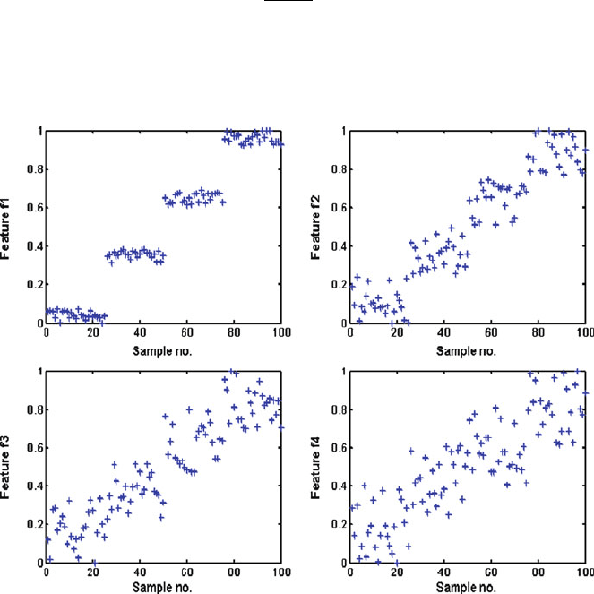
Fig. 8.4 Simulated data of ( f

, f

) for developing a feature selection scheme

132 8 Wavelet Packet Transform for Defect Severity Classiﬁcation

Y ¼ A

pq

X (8.20)

where q<p, and A

pq

is the ﬁrst q columns of A.

Given that the features transformed by the principal components are not directly

connected to the physical nature of the defect, the eigenvectors in A

pq

for the

transformed features are only used as the basis for choosing the most signiﬁcant

features from the original p-dimensional feature vectors. This is explained by

means of a numerical simulation. As illustrated in Fig. 8.4, four normalized feature

vectors, f

, f

, and f

, are constructed with each of them forming clusters around

four distinct levels of magnitudes. A total of 100 samples are considered for each of

the four features, hence each feature is a 100-by-1 vector. The four features are

simulated to have random variations from the same mean for each of the four

clusters. This is similar in principle to the variation of a measured data feature for

four different defect severities. Each of the four clusters for each feature contained

25 data points. The four features become less clearly differentiated from f

to f

,as

overlap between the clusters increases.

It is evident that a suitable feature selection scheme should be able to rank f

, f

, and f

in the same order as shown in Fig. 8.4. To derive the principal components

for the simulated data set, the four normalized features are collected in a 4-by-100

matrix X:

X ¼½f

; f



(8.21)

The eigenvalues and the eigenvectors are calculated from the scatter matrix S.The

matrix of eigenvectors can be represented as A ¼[a

i,j

], where i ¼1to4,andj ¼1to4.

The eigenvector a

consists of four components from the fourth column of the matrix

A as a

¼½

1;4

2;4

3;4

4;4

. Similar arrangement applies to a

, a

,anda

(i.e.,

¼½

1;1

2;1

3;1

4;1

, a

¼½

1;2

2;2

3;2

4;2

,and

¼½

1;3

2;3

3;3

4;3

 ), respectively. The matrix A is a 4  4 square matrix

because of the presence of the four features f

. The eigenvector corresponding to the

eigenvalue with the largest magnitude is chosen. As shown in Table 8.2, one of the

four eigenvalues of the data set is much larger than the other three, indicating that most

of the variance is concentrated in one direction. Table 8.3 lists the component

magnitudes for the eigenvector corresponding to the largest eigenvalue. Since this

corresponds to a

, the feature that is responsible for the maximum variance in the data

is thus identiﬁed.

Subsequently, the magnitudes of the four components of e

are examined. As

shown in Table 8.3, ja

1,4

j > ja

2,4

j > ja

3,4

j > ja

4,4

j. This result can be interpreted in

terms of the directionality of the eigenvector (a

) in the original feature space. If the

unit vectors for the original feature space are represented as u

, u

, and u

(where

¼ [1 0 0 0]

, u

¼ [0 1 0 0]

, etc.), then a higher magnitude of a

i,4

denotes

the similarity in direction of the eigenvector a

with u

, when compared with the

other unit vectors forming the basis for the original feature space. For the simulated

data, the component a

1,4

has the largest magnitude, followed by a

2,4

, a

3,4

, and a

4,4

8.2 Key Feature Selection 133

Thus, the feature represented along u

is the most sensitive, followed by those along

, u

, and u

. As a result, the PCA-based scheme ranks the four features f

desired and selects most representative features.

8.3 Neural-Network Classiﬁer

Once a suitable feature set (e.g., 6) is chosen from the extracted features (e.g., 32),

the machine defect severity levels can be evaluated by means of a status classiﬁer.

Neural network as a classiﬁer has been applied to machine health diagnosis, for

example, for classifying rotating mac hines with imbalance and rub faults (McCor-

mick and Nandi 1997), bearing faults (Li et al. 2000), and tank reactor operation

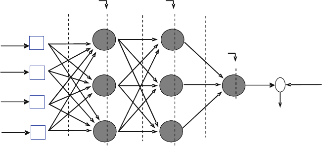
states (Maki and Loparo 1997). In general, a neural network consists of multiple

layers of nodes or neurons, and each layer has a number of parallel nodes that are

connected to all the nodes in the succeeding layer through different weights

(Haykin 1994). Using a training algorithm, the weights are adjusted such that the

neural network responds to the inputs with outputs corresponding to the severity of

a structura l defect at the output layer. Figure 8.5 illustrates the architecture of a

feed-forward neural network. For the ith layer of links, the symbols w

(i)

, b

(i)

, x

(i)

and y

(i)

represent a vector of weights between the layers, node biases of a layer,

inputs of nodes at one layer, and output at the output layer, respectively. At the

output layer, a linear neuron is used to produce an output to indicate the machine

defect severity level.

The weights of a multilayer feed-forward neural network are continuously

updated, while it is trained with training data consist ing of a set of machine defect

feature input vectors (x) and known output (d). This is realized by minimizing the

error between the computed output of the network and the known output in the

training process. Consider n pairs of input and output training data {(x

, d

)j, p ¼ 1,

2,..., n}. For the pth pair data {x

, d

}, the mean square error (MSE) of the network

output y

is expressed as:

Table 8.3 The fourth

eigenvector component

magnitudes for simulated

data

Component Magnitude

1,4

0.599

2,4

0.523

3,4

0.439

4,4

0.417

Table 8.2 Eigenvalues for

simulated data

0.241

0.775

1.318

32.023

134 8 Wavelet Packet Transform for Defect Severity Classiﬁcation

m¼1

ðd

 y

(8.22)

where m is the number of nodes at the output layer. Assuming that each input vector

corresponds to a single severity value, the value of m is 1. For the entire training

data set, the total error Err, i.e., the learning error, is expressed as:

Err ¼

p¼1

m¼1

ðd

 y

(8.23)

In the training process, the learning error is minimized through continuously

updating the connection weights in its structure with certain lea rning rule. After

training with the training data, the designed network with the resulting connection

weights generalize the relationship between the input and output to correctly

classify new input data. When input feature vectors associated with a defective

measurement occur, for which the network is however not trained, the neural

network will interpola te a defect severity by the location of the new input in the

space spanned by the training data.

There are several gradient-based learning rules to minimize the learning error Err

by changing the connection weight w of the multilayer feed-forward neural network.

Different learning rules differ in how they use the gradients to update the weights w in

training. Steepest decent with ﬁxed learning rate is the traditional learning rule of the

neural network, in which the weight w

(k)

between the kth layer and (k þ 1)th layer is

tuned for each epoch, along the gradient direction by an amount:

Input Layer

(1)

Hidden Layer

(2)

Hidden Layer

(3)

Output Layer

(4)

(1)

(2)

(3)

(1)

Input

Vector x

Computed

Output

(y)

Weights

(3)

Weights

(2)

Weights

(1)

Bias

(1)

Bias

(2)

Bias

(3)

Known

Output

(d)

Error

(e)

Fig. 8.5 Structure of a multilayer feed forward neural network

8.3 Neural Network Classiﬁer 135

ðkÞ

¼ 

ðkÞ

(8.24)

where , referred to as the learning rate, is ﬁxed between 0 and 1. The learning rate

affects the convergence speed and stability of the weights during learning. Gener-

ally, the training error decreases slowly with a learning rate  close to 0. On the

contrary, the error may oscillate and not converge if  is close to 1. To speed up the

training process for the steepest descent method, (8.24) is modiﬁed by adding a

momentum term (Haykin 1994), expressed as:

ðkÞ

¼ 

ðkÞ

þ a  Dw

(8.25)

where Dw

is the previous adjust amount, and the momentum constant a is set

between 0.1 and 1 in practice. The addition of this momentum term smoothes weight

updating and tends to resist erratic weight changes (Haykin 1994). After the network is

trained with representative data, it is able to evaluate the new measurement data and

classify them according to the rules that it has learned through the training data set.

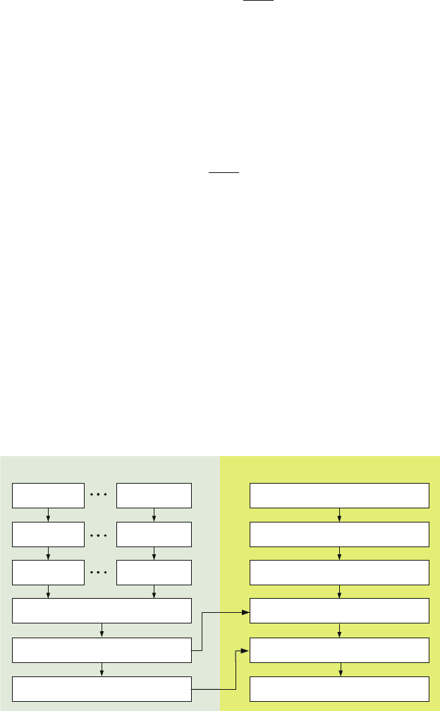
8.4 Formulation of WPT-Based Defect Severity Classiﬁcation

Utilizing the advantages of the WPT in subband signal decomposition, this section

introduces a WPT-based defect severity classiﬁcation algorithm, with assistance from

the neural-network classiﬁer introduced in Sect. 8.3. It starts with a WPT on the

measured signals. After statistical features are extracted from the wavelet coefﬁcients

Signal 1

WPT

Sub-band FE

Sub-band Feature Vectors

Signal n

WPT

Sub-band FE

Key Feature Selection

Neural Network Classifier

Wavelet Packet Transform (WPT)

Input Signal x

Neural Network (NN) Classifier

Output Diagnostic Information

Selected Feature Vector (FV)

Training Evaluation

Sub-band Feature Extraction (FE)

Store NN

Model

Guide FV

selection

Fig. 8.6 Procedure of the WPT based defect severity classiﬁcation

136 8 Wavelet Packet Transform for Defect Severity Classiﬁcation

in each subband, key feature selection process is performed to determine the most

signiﬁcant features from the feature set, which are subsequently used as input to a

neural network-based classiﬁer for defect severity classiﬁcation. Figure 8.6 illustrates

how the developed technique is realized. The left side of Fig. 8.6 depicts the training

process of the hybrid technique in a manner of supervised learning (i.e., based on the

available reference data, denoted as signal 1, ..., n). In addition to providing inputs

for constructing the neural-network classiﬁer model, the results from the feature

selection process are used to guide the feature vector selection in the evaluation

process. The right side of Fig. 8.6 describes an evaluation process of the WPT-based

algorithm. An input signal is passed through the process of signal decomposition,

feature extraction, and selection. Eventually, the corresponding defect severity level

is determined through the neural network classiﬁer.

8.5 Case Studies

The appl ication of the above described wavelet packet-based machine defect

severity classiﬁcation algorithm is described through two case studies.

8.5.1 Case Study I: Roller Bearing Defect Severity Evaluation

The ﬁrst case study is to evaluate the defect severity level of a set of roller bearings

(N205 ECP) with and without seeded defects. Speciﬁcally, vibration data were

measured from both a new, “healthy” bearing that served as a reference base and

three defective bearings containing localized defects of different sizes:

(a) one 0.1 mm diameter hole in the outer raceway

(b) one 0.5 mm diameter hole in the outer raceway

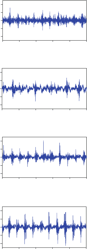
In Fig. 8.7, segments of vibration signals measured from the healthy and defective

bearings are shown.

To provide sufﬁcient training and testing data sets to the neural-network classi-

ﬁer, a total of 240 vibration data sets were collected under a bearing rotating

speed of 1,200 rpm and a radial load of 3,600 N. For each operation condition,

60 data sets were collected. Each data set was ﬁrst decomposed by the WPT.

Analysis has shown that features extracted from a four-level decomposition

provided adequate information to differentiate the four defect conditions from

each other (Gao and Yan 2007). On the basis of the information collected in the

16 subfrequency bands (since 2

¼ 16 ), a feature vector was subsequently con-

structed, which contained 32 feature elements (i.e., 16 subband energy values and

16 subband kurtosis values).

8.5 Case Studies 137

FLD analysis is then applied for feature selection . The means and variances of the

feature element, f

, are obtained for each of the four bearing conditions. Table 8.4

summarizes the discriminant power of the extracted features for different condition

pairs, based on the Fisher discriminant criterion. The ﬁrst three key features within

each condition pair, for example, E

, E

, and E

for the condition pair (healthy,

light defect), are selected, and the ﬁnal feature set is obtained through a union

0 20406080100

0.4

0.2

−0.4

−0.2

Time (ms)

Signal (V)

Signal from a healthy bearing

0 20406080100

0.4

0.2

−

0.4

−

0.2

Time (ms)

Signal (V)

Signal from a defective bearing (0.1 mm diameter hole)

0 20406080100

0.4

0.2

−0.4

−0.2

Time (ms)

Signal (V)

Signal from a defective bearing (0.5 mm diameter hole)

0 20 40 60 80 100

0.4

0.2

−0.4

−0.2

Time (ms)

Signal (V)

nal from a defective bearin

(1 mm diameter hole)

Fig. 8.7 Vibration signals

measured from roller bearings

with different conditions. (a)

Signal from a healthy bearing.

(b) Signal from a defective

bearing (0.1 mm diameter

hole). (c) Signal from a

defective bearing (0.5 mm

diameter hole). (d) Signal

from a defective bearing

(1 mm diameter hole)

138 8 Wavelet Packet Transform for Defect Severity Classiﬁcation

operation from all the six condition pairs as listed in Table 8.5, where the energy

features E

, E

, and E

are selected as the most repr esentative

features, because they possess higher discriminant power than others as listed in

Table 8.4.

Next, the PCA technique was performed on the feature vectors. As seen in Fig. 8.8,

the ﬁrst ﬁve principal components represent over 90% variance, which preserves most

of the information contained in the original feature set (Jolliffe 1986). This is

Table 8.4 Discriminant power of the extracted features for various condition pairs in different

subbands

Subband

features

Healthy vs.

light

Healthy vs.

medium

Healthy vs.

severe

Light vs.

medium

Light vs.

severe

Medium

vs. severe

0.52 2.55 1.80 2.58 2.19 2.15

0.06 48.91 8.57 0.43 0.05 10.49

18.29 695.40 118.62 41.28 8.37 193.98

0.01 110.73 8.86 1.06 0.97 27.86

1,222.60 92.10 89.62 1,696.00 216.26 52.50

45.20 212.92 125.51 374.81 260.53 11.15

41.60 346.97 61.40 2.88 0.08 5.64

226.86 440.07 191.23 308.11 88.32 71.01

2.41 172.13 7.43 173.16 0.01 183.39

87.38 47.61 4.48 69.18 204.47 52.60

466.15 8.60 211.70 916.98 170.90 340.01

80.74 14.86 69.41 60.15 15.69 44.79

5,118.80 1,238.00 133.33 7,946.10 873.16 12.21

12,702.00 308.19 2,280.10 7,397.60 3,293.60 788.82

3,652.80 36.25 2,374.40 2,414.90 707.70 1,414.70

1,863.40 56.36 12,956.60 730.50 86.52 1,150.90

2.54 57.50 41.34 0.33 0.10 7.88

0.01 0.33 4.04 0.01 0.01 2.30

0.02 17.60 7.80 0.03 0.01 16.22

0.04 6.98 37.80 0.04 0.03 51.64

0.91 39.95 9.99 0.03 0.25 3.07

0.34 74.66 50.31 0.18 0.15 1.06

0.07 2.33 7.47 0.09 0.10 8.72

7.81 30.13 21.94 1.84 1.90 10.41

0.98 51.73 6.09 0.05 0.14 0.36

0.40 74.16 32.09 0.10 0.18 7.43

0.25 14.71 9.05 0.02 0.06 0.51

0.89 15.32 38.21 0.11 0.38 3.09

0.30 4.62 11.99 0.04 0.02 0.93

0.02 9.95 2.88 0.01 0.02 0.92

0.03 16.09 3.15 0.02 0.03 2.39

0.01 9.42 4.90 0.01 0.01 1.51

8.5 Case Studies 139