Gao R.X., Yan R. Wavelets: Theory and Applications for Manufacturing

Подождите немного. Документ загружается.

0 0.005 0.01 0.015 0.02

−2

−1

Time (s)

Vsensor (Volts)

0 0.005 0.01 0.015 0.02

−2

Time (s)

Vsensor (Volts)

Original signal

Filtered signal, stopband = 1500 Hz

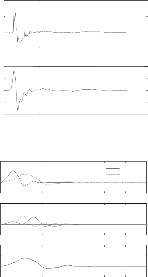
Fig. 11.3 Impulse response of a ball bearing

−

0 2 4 6 8 10 12 14

−

0 2 4 6 8 10 12 14

0 2 4 6 8 10 12

−

f(t)

f(t/2)

–0.5

f(t – n), n = 0, 1, …, 7

–0.5

f(t/2) = Σh

f(t – n)

Fig. 11.4 The Daubechies scaling function

11.2 Construction of an Impulse Wavelet 193

After the sequence of coefﬁcients h

is obtained, they are used to form an FIR

ﬁlter denoted by H

. The FIR ﬁlters H

and G

are quadrature mirror ﬁlters if, for a

signal x(t):

jjH



xðtÞjj þ jjG



xðtÞjj ¼ jjxðtÞjj (11.4)

Together, H

and G

form a pair of reconstruction ﬁlters for the wavelet decompo-

sition of a signal. This process, called deconstruction , is implemented via the

adjoints of H

and G

, which are denoted by H and G, respectively (Kaiser 1994).

For the Daubechies scaling function f(t) shown in Fig. 11.4a, the ﬁlter coefﬁcients

are as follows: h

¼ {0.2304, 0.7148, 0.6309, 0.0280, 0.1870, 0.0308, 0.0329,

0.0106}, n ¼ 0, 1, . . . , 7 (Misiti et al. 1997). In Fig. 11.4b, the scaled and

translated version of f(t) (i.e., h

f(t n) for n ¼ 0, 1, 2, . . . , 7) is shown. Since

f(t) is a valid scaling function and h

are valid ﬁlter coefﬁcients, the dilation

equation is satisﬁed, as shown in Fig. 11.4c.

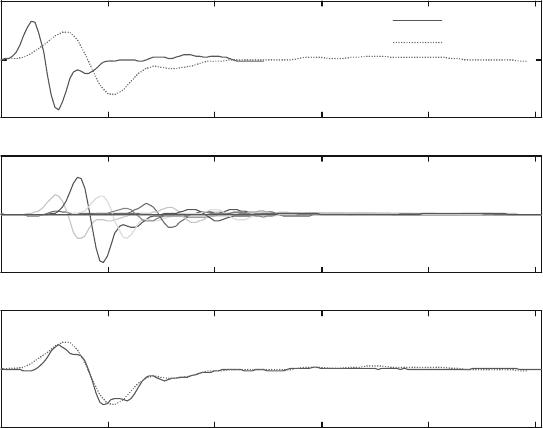
The above procedure is repeated for the impulse response as shown below in

Fig. 11.5. It should be noted that the impulse response f(t) here is a function of the

bearing dynamics, not an exact solution to the dilation equation . However, a set of

ﬁlter coefﬁcients h

can be determined such that the impulse response approxi-

mately satisﬁes the dilation equation.

The ﬁlter coefﬁcients can be calculated such that the dilation equation is sat isﬁed

exactly at integer values of t. The solution is recursive: each h

, for n > 0, can be

0 5 10 15 20 25

−

0 5 10 15 20 25

−

0 5 10 15 20 25

−

φ(t)

–0.5

φ(t/2)

φ(t – n), n = 0, 1, …, 12

–0.5

φ(t/2) = Σh

φ(t – n)

Fig. 11.5 The impulse scaling function obtained from the ball bearing

194 11 Designing Your Own Wavelet

explicitly determined as a function of f(t) and h

, h

,..., h

n 1

.Theﬁrst

coefﬁcient, h

, is simply a function of f(t). These solutions are obtained by eval-

uating the dilation equation at integer values of t.Fort ¼ 1, (11.1)gives

fð1=2Þ= 2

¼ h

fð1Þ. The terms h

fð0Þ, h

fð1Þ, etc., do not appear because

f(t) ¼ 0fort  0. (Recall that f is compactly supported.) Thus, h

is determined by:

fð1=2Þ

fð1Þ

(11.5)

Similarly, for t ¼ 2, (11.1) gives:

fð1Þ¼h

fð2Þþh

fð1Þ (11.6)

For t ¼ 3:



¼ h

fð3Þþh

fð2Þþh

fð1Þ (11.7)

For t ¼ N +1:

N þ 1



¼ h

fðN þ 1Þþh

fðNÞþh

fðN  1Þþþh

fð1Þ (11.8)

Equations (11.5) (11.8) determine a recursive deﬁnition for each ﬁlter coefﬁcient h

With the ﬁrst coefﬁcient h

given by (11.5), the remaining coefﬁcients are given by:

1=2

fððn þ 1Þ=2Þ

n 1

k 0

fðn þ 1  kÞ

fð1Þ

; for n  1 (11.9)

Since the scalin g function f(t) is given by the impulse response of the bearing, each

of the ﬁlter coefﬁcients h

can be readily determined from (11.5) and (11.9).

Furthermore, note that the dilation equation can be written as:



¼ h

fðtÞþ

j¼1

fðt  jÞ (11.10)

Since h

is given by (11.9), the dilation equatio n can be rewritten as:



j 1

1=2

fððj þ1Þ=2Þ

j 1

k 0

fðj þ1 kÞ

fðt jÞ

fð1Þ

þh

fðtÞ (11.11)

11.2 Construction of an Impulse Wavelet 195

Collecting terms yields the following form for the dilation equation:



j 1

½2

1=2

fððj þ 1Þ=2Þfðt  j Þ

fð1Þ



j 1

k 0

fðj þ 1  kÞfðt  jÞ

fð1Þ

þ h

fðtÞ (11.12)

Note that only the second term on the right hand side of (11.12) contains ﬁlter

coefﬁcients h

, which are determined by (11.5) and (11.9). Equation (11.12) serves

to illustrate the interesting relationship that the dilation equation imposes between

and f(t). Particularly, the expression given by (11.12) shows that the dilated

version of the scaling functi on is related not only to f(t  n) scaled by the ﬁlter

coefﬁcient h

, but also to f(t  n), scaled by f(t), which is evaluated at integer

values of t. The recursive relationship given by (11.9) gives h

such that the dilation

equation is satisﬁed at x ¼ {0, 1, 2, . . .}. At other points, the sum on the right hand

side of (11.1) might differ from the left hand side. In practical treatment of an

impulse scaling function such as shown in Fig. 11.5a, (11.5) and (11.9) are ﬁrst used

to obtain an initial set o f ﬁlter coefﬁcients. These coefﬁcients are then optimized by

minimizing the following error function:

rms





fðt  nÞ

(11.13)

The error E

rms

is a scalar valued function of the vector of ﬁlter coefﬁcients h

, and the

optimization is accomplished by ﬁnding the vector which minimizes E

rms

. Since

rms

is a measure of how well the dilation equation is satisﬁed, the vector h

minimizing E

rms

is the best set of ﬁlter coefﬁcients that can be obtained from f(t).

Using this technique, the ﬁlter coefﬁ cients are determined to be: h

¼ {0.0529,

0.4897, 0.9601, 0.4848, 0.1467, 0.2653, 0.1723, 0.1295, 0.1208, 0.0495, 0.0182,

0.0255, 0.0131}, for n ¼ 0, 1, . . . , 12. The translated and scaled versions of f(t)

corresponding to these h

(i.e., h

f(t  n)) are plotted in Fig. 12.5b. As indicated by

Fig. 12.5c, the impulse response is an approximate solution to the dilation equation

rms

¼0.0984). The low pass ﬁlter coefﬁcients derived from this scaling function f(t)

can then be used to determine the corresponding wavelet c(t)(Young1993;Mallat

1998). The coefﬁcients for the high pass reconstruction ﬁlter G

are determined from

(11.4). The wavelet is evaluated by upsampling G

, convolving it with H

, and then

iteratively repeating this procedure:



nþ1

¼* G



H



(11.14)

where * is a dyadic up-sampling operator. Thus, after N iterations, cðtÞﬃH



Nþ1

Figure 11.6 shows the result of four iterations of (11.1 4 ), which produced a

196 11 Designing Your Own Wavelet

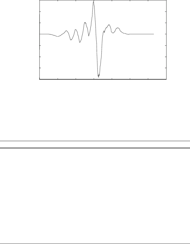
customized wavelet, based on the impulse response of the rolling bearing structure.

The set of FIR ﬁlters based on c(t) and synthesis based on f(t) are given in

Table 11.1, where the ﬁlters have been normalized to have a norm of 1= 2

0.15

0.1

0.05

0.1

0.15

0.2

0 2 4 6 8 10 12

Amplitude

Fig. 11.6 The wavelet derived from the impulse response

Table 11.1 Normalized ﬁlter coefﬁcients

Deconstruction Reconstruction

Low pass High pass Low pass High pass

0 0.0274 0.0274 0

0.0068 0.2532 0.2532 0.0068

0.0132 0.4964 0.4964 0.0132

0.0094 0.2507 0.2507 0.0094

0.0256 0.0759 0.0759 0.0256

0.0625 0.1372 0.1372 0.0625

0.0670 0.0891 0.0891 0.0670

0.0891 0.0670 0.0670 0.0891

0.1372 0.0625 0.0625 0.1372

0.0759 0.0256 0.0256 0.0759

0.2507 0.0094 0.0094 0.2507

0.4964 0.0132 0.0132 0.4964

0.2532 0.0068 0.0068 0.2532

0.0274 0 0 0.0274

11.2 Construction of an Impulse Wavelet 197

11.3 Impulse Wavelet Application

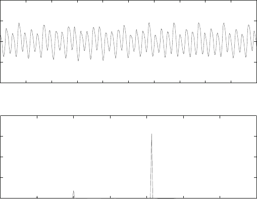
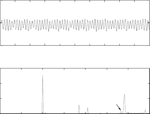
As an application example, the impulse wavelet is used to diagnose bearing defect.

Figure 11.7a shows a vibration signal measured on a SKF 6220 ball bearing with a

0.25-mm hole on its inner raceway. This signal is sampled at 10 kHz, and the

rotating speed of the bearing is 600 rpm (i.e., corresponding to 10 Hz rotating

frequency). Based on geometric dimensions of the bearing and the rotating speed

(Harris 1991), the defect characteristic frequency on the inner raceway of such

bearing is f

BPFI1

¼ 58.6 Hz. As illustrated in Fig. 11.7b, such a defect-related

frequency component is not seen in its power spectral density (PSD) resulted from

the Fourier transform.

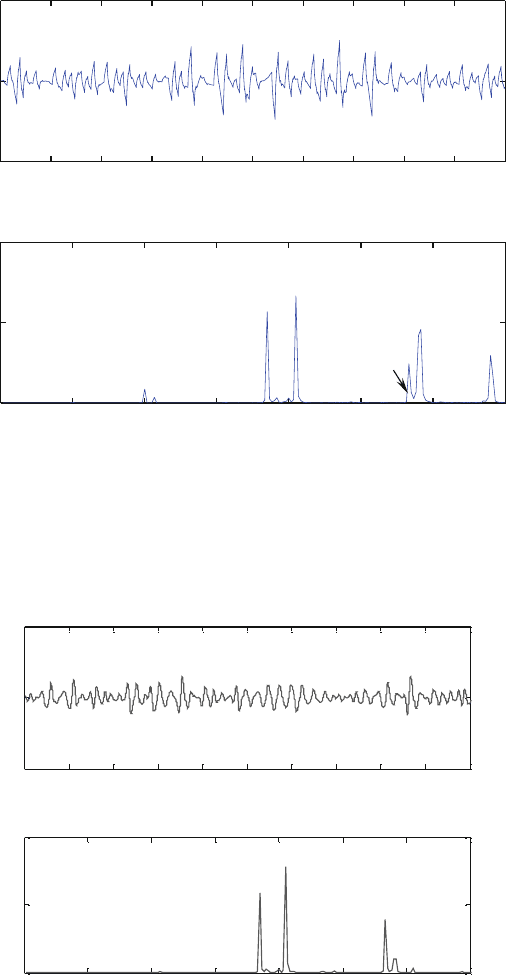
Utilizing the wavelet integrated with Fourier transform technique, which is

described in Chap. 7, the same vibration signal is ﬁrst analyzed by the wavelet

transform. The impulse wavelet, developed from the impulse response of the rolling

bearing as described above, is used as the base wavelet. Fourier transform is then

performed on the wavelet coefﬁcients obtained from the wavelet transform to

expose explicitly the related frequency components. Figure 11.8 illustrates the

resulting wavelet coefﬁcients and their corresponding PSD. It is seen that the

defect-related frequency component f

BPFI1

at 58.6 Hz is clearly shown in the

spectrum, thus verifying the existence of a localized inner raceway defect.

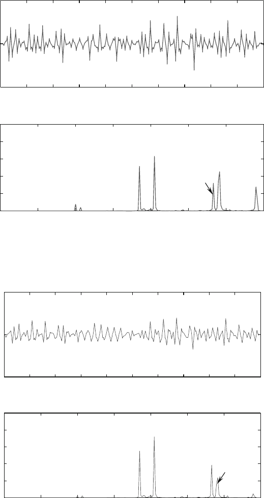
To demonstrate the signature extraction capability of the designed impulse

wavelet for bearing defect diagnosis, a comparison study is carrie d out, where

0 0.1 0.2 0.3 0.4 0.5 0.6 0.7 0.8 0.9 1

−1

−0.5

0.5

Time (s)

Signal (V)

10 20 30 40 50 60 70

0.02

0.04

0.06

0.08

Frequenc

(Hz)

PSD (Watts/Hz)

BPFO1

Fig. 11.7 Vibration signal and its PSD from a defective bearing

198 11 Designing Your Own Wavelet

ﬁve standard base wavelets from the literature: Daubechies 2 and 4 wavelets,

Coiﬂets 1, Symlets 3, and Biorthogonal 2.2 (Daubechies 1992 ; Lou and Loparo

2004; Zhang et al. 2005) are used to analyze the vibration signal. The upper parts of

Figs. 11.9 11.13 are intermediate results (i.e., wavelet coefﬁcients) of the

integrated wavelet-Fourier transf orm analysis, and the lower parts of these ﬁgures

are their corresponding PSDs. It is shown that all the ﬁve standard base wavelets

can identify the defect-related frequency component, and the results are shown in

the lower parts of Figs. 11.9 11.13.

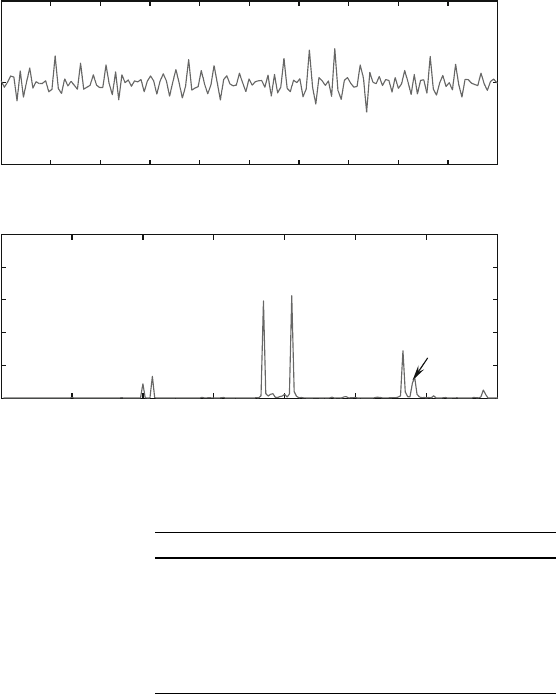
In the spectra of Figs. 11.9 11.13, there exists a frequency component f

BPFO2

56.5 Hz, which has a distinct magnitude. Such a frequenc y component is identiﬁed

as from the ball rotation of another bearing in the support structure (Yan et al.

2009). To enabl e a quantitative performanc e comparison of the developed impulse

wavelet and other ﬁve standard base wavelets, a sign al-to-noise ratio measure is

introduced, which is the amplitude ratio between the defect frequency f

BPFI1

and the

adjacent frequency f

BPFO2

. As listed in Table 11.2, the impulse wavelet has shown

the highest signal-to-noise ratio in detecting the defect-characteristic frequency of

BPFI1

¼ 58.6 Hz. This result can be attributed to the nature of this customized

wavelet, which is derived from the actual impulse respo nse of the bear ing structure.

The direct link to the dynamics of the bearing and thus inherent better match to the

bearing signature than a standard wavelet has made it more effective in exposing

the constituent features for defect identiﬁcation.

0 0.1 0.2 0.3 0.4 0.5 0.6 0.7 0.8 0.9 1

−0.05

0.05

Time (s)

Signal (V)

0 10203040506070

0.5

1.5

x 10

−6

Frequenc

(Hz)

PSD (Watts/Hz)

BPFO1

BPFO2

BPF11

Fig. 11.8 Wavelet integrated Fourier spectrum using the customized impulse wavelet

11.3 Impulse Wavelet Application 199

0 0.1 0.2 0.3 0.4 0.5 0.6 0.7 0.8 0.9 1

−0.5

0.5

Time (s)

Signal(V)

0 10 20 30 40 50 60 70

0.5

x 10

−3

Frequency (Hz)

PSD (Watts/Hz)

BPFO1

BPFI1

BPFO2

Fig. 11.9 Wavelet integrated Fourier spectrum results using Daubechies 2 (Db2) wavelet

BPFI1

BPFO2

0 0.1 0.2 0.3 0.4 0.5 0.6 0.7 0.8 0.9 1

0.5

Time (s)

Signal (V)

0 10 20 30 40 50 60 70

0.5

x 10

−3

Frequency (Hz)

PSD (Watts/Hz)

BPFO1

Fig. 11.10 Wavelet integrated Fourier spectrum results using Daubechies 4 (Db4) wavelet

200 11 Designing Your Own Wavelet

0 0.1 0.2 0.3 0.4 0.5 0.6 0.7 0.8 0.9 1

−0.5

0.5

Time (s)

Signal (V)

0 10 20 30 40 50 60 70

0.2

0.4

0.6

0.8

x 10

−3

Frequenc

(Hz)

PSD (Watts/Hz)

BPFO1

BPFO2

BPF11

Fig. 11.11 Wavelet integrated Fourier spectrum results using Coiﬂets 1 (Coif1) wavelet

BPFO1

0 0.1 0.2 0.3 0.4 0.5 0.6 0.7 0.8 0.9 1

−0.5

0.5

Time (s)

Signal (V)

0 10 20 30 40 50 60 70

0.2

0.4

0.6

0.8

x 10

−3

Frequency (Hz)

PSD (Watts/Hz)

BPFO2

BPF11

Fig. 11.12 Wavelet integrated Fourier spectrum results using Symlets 3 (Sym3) wavelet

11.3 Impulse Wavelet Application 201

11.4 Summary

This chapter introduces the procedure to design a wavelet based on the dynamics of

the physical syst em being analyzed. Using the impulse response of a rolling bearing

system, an impulse wavelet has been constructed for defect-induced signature

extraction. Experimental study has veriﬁed the effectiveness of the impulse wavelet

in identifying bearing localized defect of the bearing in its inner raceway, as

illustrated in the comparative study involving ﬁve standard wavelets from the

literature. Although the impulse wavelet development is based on a speciﬁc type

of bearing, the analytical procedure described in this chapter should be applicable to

the analysis of other types of mechanical systems.

0 0.1 0.2 0.3 0.4 0.5 0.6 0.7 0.8 0.9 1

−0.5

0.5

Time (s)

Signal (V)

0 10 20 30 40 50 60 70

0.2

0.4

0.6

0.8

x 10

−3

Frequency (Hz)

PSD (Watts/Hz)

BPFO1

BPFI1

BPFO2

Fig. 11.13 Wavelet integrated Fourier spectrum results using Biorthogonal 2.2 (Bior2.2) wavelet

Table 11.2 Comparison of

signal to noise ratios for

different base wavelets

Base wavelet f

BPFI1/

BPFO2

Impulse 9.55

Db2 1.88

Db4 0.27

Coif1 1.41

Sym3 0.62

Bior2.2 0.43

202 11 Designing Your Own Wavelet