Gockenbach M.S. Partial Differential Equations. Analytical and Numerical Methods
Подождите немного. Документ загружается.

478
Chapter
10.
More about
finite
element methods
Figure
10.8.
The
sparsity
pattern
of
the L
(left)
and U
(right)
factors
of
the
discrete
Laplacian
(200 triangular elements).
of
the
matrix-vector
product
is
mostly governed
by the
density
of the
matrix
(the
percentage
of
nonzero
entries).
10.2.4
Iterative
solution
of
sparse
linear
systems
Even
when
A is
sparse,
it may be too
costly,
in
terms
of
arithemtic operations
or
memory
(or
both),
to
solve
Ax
=
b
directly.
An
alternative
is to use an
iterative
algorithm,
which
produces
a
sequence
of
increasingly accurate approximations
to the
true solution. Although
the
exact solution
can
generally
not be
obtained except
in
the
limit
(that
is, an
infinite number
of
steps
is
required
to get the
exact
solution),
in
many cases
a
relatively
few
steps
can
produce
an
approximate solution
that
is
sufficiently
accurate. Indeed,
we
should keep
in
mind
that,
in the
context
of
solving
differential
equations,
the
"exact" solution
to Ax
=
b is not
really
the
exact
solution—it
is
only
an
approximation
to the
true solution
of the
differential
equation.
Therefore,
as
long
as the
iterative
algorithm introduces errors
no
larger
than
the
discretization errors,
it is
perfectly
satisfactory.
Many
iterative algorithms have been developed,
and it is
beyond
the
scope
of
this book
to
survey them.
We
will
content ourselves with outlining
the
conjugate
gradient (CG) method,
the
most popular algorithm
for
solving
SPD
systems.
(The
stiffness
matrix
K
from
a finite
element problem, being
a
Gram matrix,
is
SPD—see
Exercise
6.) We
will
also
briefly
discuss preconditioning,
a
method
for
accelerating
convergence.
478
Chapter 10.
More
about finite element methods
20
40 40
60
60
80"'-
____
_
80"'-
_____
_
o
20
40
60
80
o
20
40
60
80
nz
=
737
nz
=
737
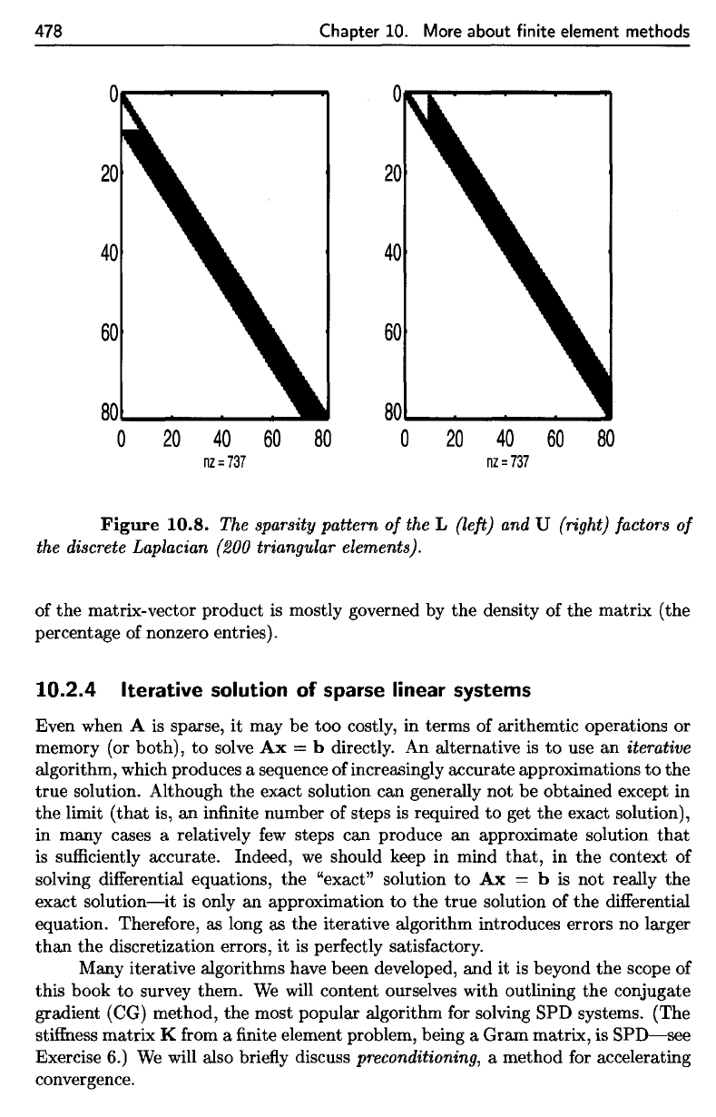
Figure
10.8.
The sparsity pattern
of
the L {left} and U {right} factors
of
the discrete Laplacian {200 triangular elements}.
of
the
matrix-vector product is mostly governed by
the
density of
the
matrix
(the
percentage of nonzero entries).
10.2.4
Iterative solution
of
sparse linear systems
Even when A is sparse,
it
may be
too
costly, in terms of arithemtic operations
or
memory (or both),
to
solve
Ax
= b directly. An alternative is
to
use
an
iterative
algorithm, which produces a sequence of increasingly accurate approximations
to
the
true
solution. Although
the
exact solution can generally
not
be obtained except in
the
limit
(that
is,
an
infinite number
of
steps is required
to
get
the
exact solution),
in many cases a relatively
few
steps can produce
an
approximate solution
that
is sufficiently accurate. Indeed,
we
should keep in mind
that,
in
the
context of
solving differential equations,
the
"exact" solution
to
Ax
= b is
not
really
the
exact
solution-it
is only
an
approximation
to
the
true
solution of
the
differential
equation. Therefore,
as
long
as
the
iterative algorithm introduces errors no larger
than
the discretization errors,
it
is perfectly satisfactory.
Many iterative algorithms have been developed, and
it
is beyond
the
scope of
this book
to
survey them.
We
will content ourselves with outlining
the
conjugate
gradient (CG) method,
the
most popular algorithm for solving
SPD
systems. (The
stiffness
matrix
K from a finite element problem, being a
Gram
matrix, is
SPD-see
Exercise 6.)
We
will also briefly discuss preconditioning, a method for accelerating
convergence.
10.2. Solving
sparse
linear
systems
479
The CG
method
is
actually
an
algorithm
for
minimizing
a
quadratic
form.
If
A
e
R
nxn
ig
SPD
and
0 :
R
n
-»
R is
denned
by
Moreover,
a
consideration
of the
second derivative matrix shows
that
this
stationary
point
is the
global minimizer
of 0 (a
quadratic
form
defined
by an SPD
matrix
is
analogous
to a
scalar quadratic
ax
2
+bx+c
with
a >
0—see
Figure
10.10).
Therefore,
solving
Ax = b and
minimizing
0 are
equivalent.
We
can
thus apply
any
iterative minimization algorithm
to 0,
and, assuming
it
works,
it
will
converge
to the
desired value
of x. A
large class
of
minimization
algorithms
are
descent
methods based
on a
line
search.
Such algorithms
are
based
on
the
idea
of a
descent
direction:
Given
an
estimate
x^
of the
solution,
a
descent
direction
p is a
direction such
that,
starting
from
x^,
0
decreases
in the
direction
of
p.
This means
that,
for all a > 0
sufficiently
small,
Figure
10.9.
A
random
sparse
matrix
(left)
and its
lower
triangular factor
(right).
then
a
direct calculation (see Exercise
3)
shows
that
Therefore,
the
unique stationary point
of 0 is
10.2. Solving sparse linear systems
479
o
50
100
nz
=
946
nz
=
3096
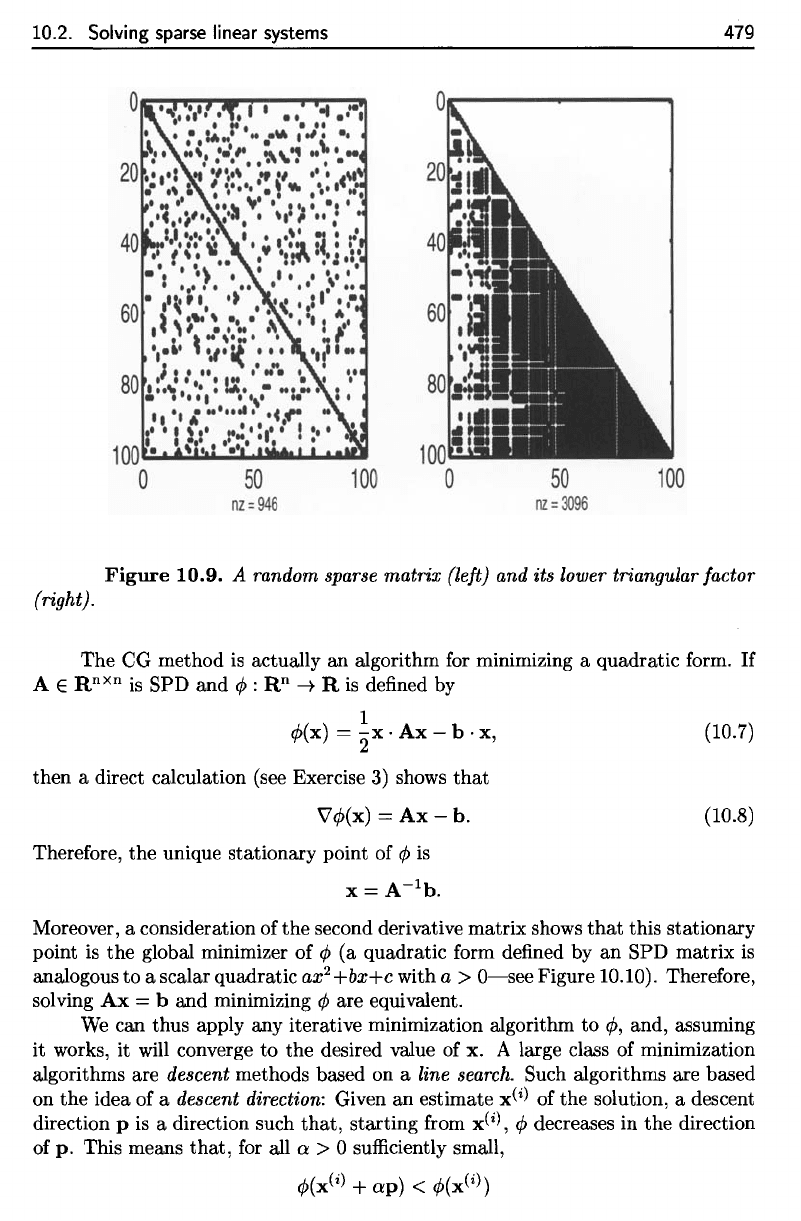
Figure
10.9.
A random sparse matrix (left) and its lower triangular factor
(right).
The
CG method
is
actually an algorithm for minimizing a quadratic form.
If
A E Rnxn is SPD
and
¢ : Rn
--t
R is defined by
1
¢(x)
= "2x.
Ax
-
b·
x, (10.7)
then
a direct calculation (see Exercise
3)
shows
that
"\l¢(x) =
Ax
- h.
Therefore,
the
unique stationary point of ¢ is
x =
A-lb.
(10.8)
Moreover, a consideration of
the
second derivative matrix shows
that
this stationary
point is
the
global minimizer of ¢
(a
quadratic form defined by
an
SPD
matrix
is
analogous
to
a scalar quadratic
ax
2
+bx+c with
a>
O-see
Figure 10.10). Therefore,
solving
Ax
= b
and
minimizing ¢ are equivalent.
We
can thus apply any iterative minimization algorithm
to
¢, and, assuming
it
works,
it
will converge
to
the
desired value of
x.
A large class of minimization
algorithms are descent methods based on a line search. Such algorithms are based
on
the
idea of a descent direction: Given
an
estimate
x(i)
of the solution, a descent
direction p is a direction such
that,
starting
from x(i), ¢ decreases in
the
direction
of
p.
This means
that,
for all a > 0 sufficiently small,
¢(x(i) +
ap)
< ¢(x(i))
480
Chapter
10.
More about
finite
element methods
Figure
10.10.
The
graph
of
a
quadratic
form
defined
by a
positive
definite
matrix.
The
contours
of the
function
are
also
shown.
holds.
Equivalently,
this means
that
the
directional derivative
of
0
at
xW
in the
direction
of p is
negative,
that
is,
Given
a
descent direction,
a
line search algorithm
will
seek
to
minimize
0
along
the
ray
(x^
+
ap
: a
>
0}
(that
is, it
will
search along this "line," which
is
really
a
ray).
Since
0
is
quadratic,
it is
particularly easy
to
perform
the
line
search—along
a
one-dimensional subset,
(j>
reduces
to a
scalar
quadratic.
Indeed,
(the symmetry
of A was
used
to
combine
the
terms
x^
•
Ap/2
and p •
Ax^/2)-
The
minimum
is
easily seen
to
occur
at
480
Chapter 10. More
about
finite element methods
6
y
x
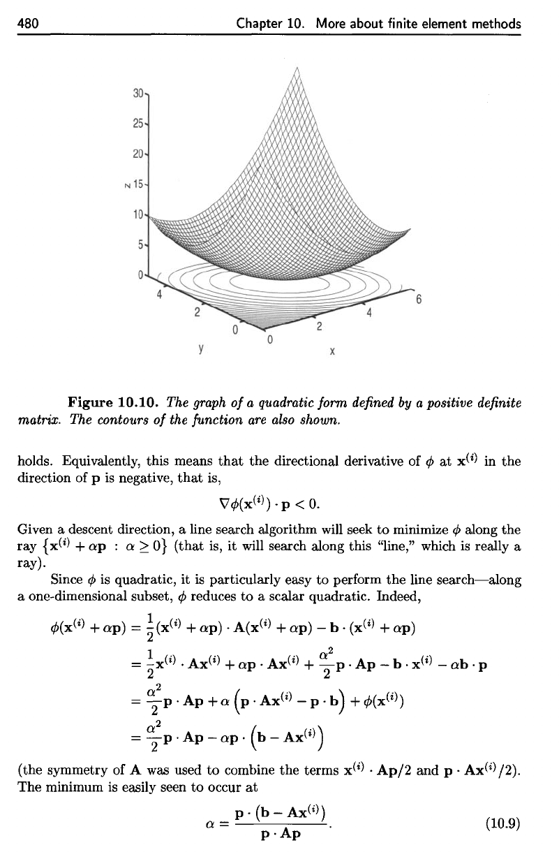
Figure
10.10.
The graph
of
a quadratic form defined
by
a positive definite
matrix. The contours
of
the junction
are
also shown.
holds. Equivalently, this means
that
the
directional derivative of ¢
at
x(i)
in the
direction of p
is
negative,
that
is,
V'¢(x(i))
. p <
O.
Given a descent direction, a line search algorithm will seek to minimize ¢ along
the
ray
{x(i)
+
ap
: a
20}
(that
is,
it
will search along this "line," which
is
really a
ray).
Since
¢ is quadratic,
it
is
particularly easy
to
perform
the
line
search-along
a one-dimensional subset, ¢ reduces
to
a scalar quadratic. Indeed,
¢(x(i)
+
ap)
=
~(x(i)
+
ap)
.
A(x(i)
+
ap)
-
b·
(x
(i) +
ap)
2
=
~x(i)
.
Ax(i)
+
ap'
Ax(i)
+ a
2
p.
Ap
-
b·
x(i)
-
ab·
p
2 2
2
=
~
p.
Ap
+ a
(p.
Ax(i)
- P .
b)
+
¢(x(i))
=
~2
p.Ap-ap.
(b-Ax(i))
(the symmetry of A was used
to
combine
the
terms
x(i)
.
Ap/2
and
p.
Ax(i)
/2).
The
minimum
is
easily seen
to
occur
at
p.
(b
-
Ax(i))
a-
--'----.:....
-
p·Ap
.
(10.9)
10.2. Solving
sparse
linear systems
481
since
the
directional derivative
of
</>
at
x^
is as
negative
as
possible
in
this direction.
The
resulting algorithm (choose
a
starting point, move
to the
minimum
in the
steepest descent direction, calculate
the
steepest descent direction
at
that
new
point,
and
repeat)
is
called
the
steepest
descent
algorithm.
It is
guaranteed
to
converge
to
the
minimizer
x of 0,
that
is, to the
solution
of Ax = b.
However,
it can be
shown
that
the
steepest descent method converges slowly, especially when
the
eigenvalues
of
A
differ
greatly
in
magnitude (when this
is
true,
the
matrix
A is
said
to be
ill-conditioned).
For an
example
of a
line search
in the
steepest descent direction,
see
Figure
10.11
and
Exercise
7.
Figure
10.11.
The
contours
of
the
quadratic
form
from
Figure
10.10.
The
steepest
descent
direction from
x =
(4,2)
(marked
by the
"o")
is
indicated,
along
with
the
minimizer
in the
steepest
descent
direction
(marked
by
"o").
The
desired
(global)
minimizer
is
marked
by
"x."
Example
10.2.
To
test
the
algorithms
described
in
this section,
we
will
use the
BVP
How
should
the
descent direction
be
chosen?
The
obvious choice
is the
steepest
descent
direction
10.2. Solving sparse linear systems
481
How should the descent direction be chosen? The obvious choice
is
the steepest
descent direction
since
the
directional derivative of ¢
at
x(i)
is
as negative as possible in this direction.
The resulting algorithm (choose a starting point, move
to
the minimum in
the
steepest descent direction, calculate the steepest descent direction
at
that
new point,
and repeat)
is
called
the
steepest descent algorithm.
It
is
guaranteed to converge
to
the
minimizer x of ¢,
that
is,
to
the solution of
Ax
=
h.
However, it can be shown
that
the
steepest descent method converges slowly, especially when
the
eigenvalues
of A differ greatly in magnitude (when this
is
true, the matrix A is said
to
be
ill-conditioned) .
For
an
example of a line search in the steepest descent direction, see Figure
10.11
and
Exercise 7.
5~--~----------~--~----~--~
4
3
o
-10~--~----~2----~3~---4~--~5----~6
x
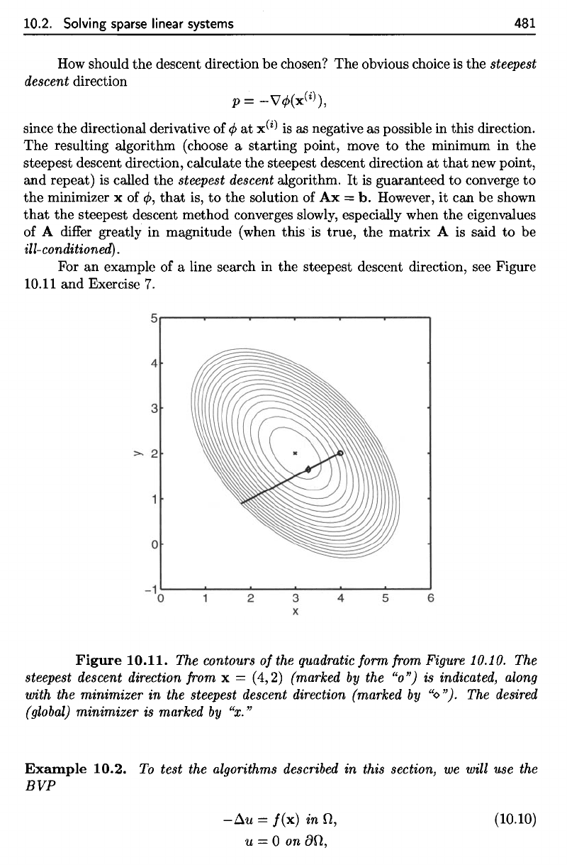
Figure
10.11.
The contours
of
the quadratic form from Figure 10.10. The
steepest descent direction from x = (4,2) (marked
by
the "0") is indicated, along
with the minimizer in the steepest descent direction (marked
by
"<:>
").
The desired
(global) minimizer is marked
by
"x."
Example
10.2.
To
test the algorithms described in this section,
we
will use the
BVP
-~u
=
f(x)
in
n,
u = 0 on
an,
(10.10)
solves
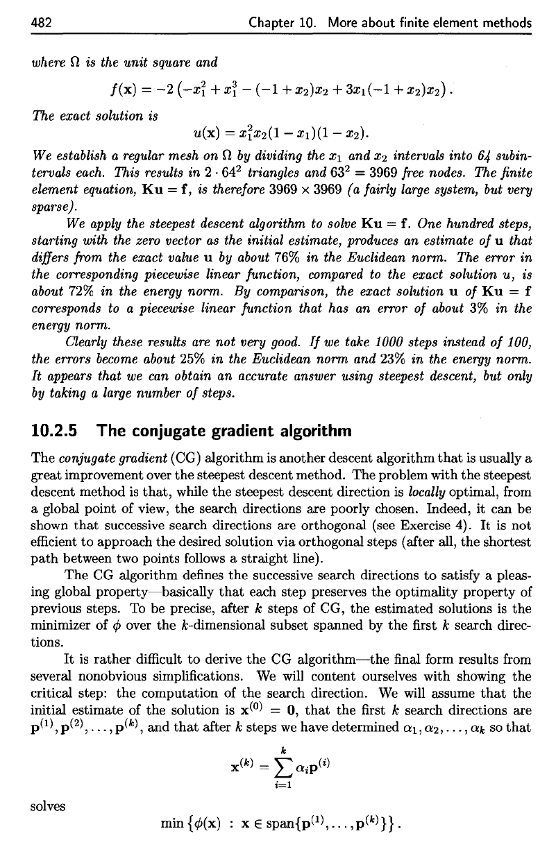
482
Chapter
10.
More about
finite
element methods
where
fi is the
unit
square
and
The
exact
solution
is
We
establish
a
regular
mesh
on
£7
by
dividing
the
x\
and
#2
intervals into
64
subin-
tervals
each.
This
results
in 2 •
64
2
triangles
and
63
2
=
3969
free
nodes.
The finite
element
equation,
Ku =
f,
is
therefore
3969
x
3969
(a
fairly
large
system,
but
very
sparse).
We
apply
the
steepest
descent
algorithm
to
solve
Ku
=
f.
One
hundred
steps,
starting
with
the
zero
vector
as the
initial estimate,
produces
an
estimate
of
u
that
differs
from
the
exact
value
u by
about
76% in the
Euclidean norm.
The
error
in
the
corresponding
piecewise
linear function,
compared
to the
exact
solution
u, is
about
72% in the
energy
norm.
By
comparison,
the
exact
solution
u
of
Ku = f
corresponds
to a
piecewise
linear function that
has an
error
of
about
3% in the
energy
norm.
Clearly
these results
are not
very
good.
If we
take 1000
steps
instead
of
100,
the
errors
become
about
25% in the
Euclidean norm
and 23% in the
energy
norm.
It
appears
that
we can
obtain
an
accurate
answer
using
steepest
descent,
but
only
by
taking
a
large
number
of
steps.
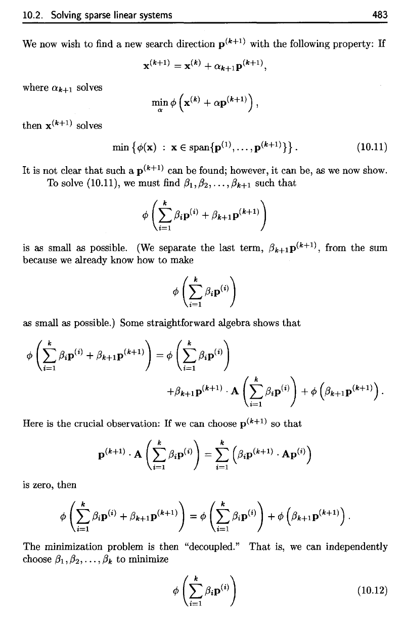
10.2.5
The
conjugate gradient algorithm
The
conjugate
gradient (CG) algorithm
is
another descent algorithm
that
is
usually
a
great improvement over
the
steepest descent method.
The
problem with
the
steepest
descent method
is
that,
while
the
steepest descent direction
is
locally
optimal,
from
a
global point
of
view,
the
search directions
are
poorly chosen. Indeed,
it can be
shown
that
successive search directions
are
orthogonal (see Exercise
4). It is not
efficient
to
approach
the
desired solution
via
orthogonal steps
(after
all,
the
shortest
path
between
two
points
follows
a
straight
line).
The CG
algorithm
defines
the
successive search directions
to
satisfy
a
pleas-
ing
global
property—basically
that
each step preserves
the
optimality property
of
previous
steps.
To be
precise,
after
k
steps
of CG, the
estimated solutions
is the
minimizer
of 0
over
the
/^-dimensional
subset spanned
by the first k
search direc-
tions.
It is
rather
difficult
to
derive
the CG
algorithm—the
final
form
results
from
several nonobvious simplifications.
We
will
content ourselves with showing
the
critical step:
the
computation
of the
search direction.
We
will
assume
that
the
initial estimate
of the
solution
is
x^°^
= 0,
that
the first k
search directions
are
p(i)
?
p(2)
^ ^
p(fc)
^
^d
t
na
t
after
k
steps
we
have determined
ai,
0:2,
• •
•,
&k
so
that
482
Chapter 10. More
about
finite element methods
where n is the
unit
square and
f(x)
=
-2
(-xi +
x~
-
(-1
+
X2)X2
+
3X1(-1
+ X2)X2).
The exact solution is
u(x)
=
xix2(1-
x1)(1-
X2).
We establish a regular mesh on n
by
dividing the
Xl
and
X2
intervals into
64
subin-
tervals
each.
This results in 2 . 64
2
triangles and 63
2
= 3969 free nodes. The finite
element equation,
K u =
f,
is therefore 3969 x 3969
(a
fairly large system, but very
sparse).
We apply the steepest descent algorithm to solve
Ku
= f. One hundred steps,
starting with the zero vector
as
the initial estimate, produces an estimate
of
u that
differs from the exact value
u
by
about
76%
in the Euclidean norm. The error in
the corresponding piecewise linear function, compared to the exact solution
u,
is
about
72%
in the energy norm.
By
comparison, the exact solution u
of
Ku
= f
corresponds to a piecewise linear function that has an error
of
about
3%
in the
energy norm.
Clearly these results
are
not
very
good.
If
we
take 1000 steps instead
of
100,
the errors become about
25%
in
the Euclidean norm and
23%
in the energy norm.
It
appears that
we
can obtain an accurate answer using steepest descent, but only
by
taking a large number
of
steps.
10.2.5 The conjugate gradient algorithm
The
conjugate gradient (CG) algorithm is another descent algorithm
that
is
usually a
great improvement over
the
steepest descent method.
The
problem with
the
steepest
descent method
is
that,
while
the
steepest descent direction is locally optimal, from
a global point of view,
the
search directions are poorly chosen. Indeed,
it
can be
shown
that
successive search directions are orthogonal (see Exercise 4).
It
is
not
efficient
to
approach
the
desired solution via orthogonal steps (after all,
the
shortest
path
between two points follows a straight line).
The
CG algorithm defines
the
successive search directions
to
satisfy a pleas-
ing global
property-basically
that
each step preserves the optimality property of
previous steps. To be precise, after
k steps of CG,
the
estimated solutions is
the
minimizer of ¢ over the k-dimensional subset spanned by
the
first k search direc-
tions.
It
is
rather
difficult
to
derive
the
CG
algorithm-the
final form results from
several nonobvious simplifications.
We
will content ourselves with showing
the
critical step:
the
computation of
the
search direction.
We
will assume
that
the
initial estimate of
the
solution is
x(O)
= 0,
that
the first k search directions are
p(l),
p(2),
...
,p(k), and
that
after k steps
we
have determined
a1,
0:2,
...
,ak
so
that
k
x(k)
= L
aiP(i)
i=l
solves
min
{¢(x)
x E span{p(1),
...
,p(k)}} .
10.2. Solving
sparse
linear
systems
483
We
now
wish
to find a new
search direction
p(
fe+1
)
with
the
following
property:
If
where
ctk+i
solves
then
x(
fc+1
)
solves
It is not
clear
that
such
a
p(
fc+1
)
can be
found;
however,
it can be, as we now
show.
To
solve
(10.11),
we
must
find
/?i,
/9
2
,
• •
•,
0k+i
such
that
is
as
small
as
possible.
(We
separate
the
last
term,
0k+ip(
k+1
\
from
the sum
because
we
already know
how to
make
as
small
as
possible.) Some straightforward algebra shows
that
Here
is the
crucial observation:
If we can
choose
p(
fc+1
)
so
that
is
zero, then
The
minimization problem
is
then
"decoupled."
That
is, we can
independently
choose
8-1.
8<>
81.
to
minimize
10.2. Solving sparse linear systems
483
We
now wish
to
find a new search direction p(k+
1
)
with the following property:
If
x(k+1)
=
x(k)
+
ak+lp(k+1)
,
where
ak+l
solves
then x(k+
1
)
solves
min
{¢>(x)
: x E span{p(1),
...
,p(k+1)}} .
(10.11)
It
is
not clear
that
such a
p(k+1)
can be found; however,
it
can be, as
we
now show.
To
solve
(1O.11),
we
must find
f31,/h
...
,f3k+1 such
that
is
as small as possible.
(We
separate the last term,
f3k+1p(k+
1
),
from the sum
because
we
already know how
to
make
as small as possible.) Some straightforward algebra shows
that
¢>
(t,
f3iP(i) +
f3k+lP(k+1))
=
¢>
(t,
f3iP(i))
+f3k+lP(k+
1
) .
A
(t,
f3iP(i)) +
¢>
(f3k+
1
P(k+1))
.
Here
is
the
crucial observation:
If
we
can choose
p(k+1)
so
that
is
zero, then
The minimization problem
is
then "decoupled."
That
is,
we
can independently
choose
f31, f32,
...
,f3k to minimize
(10.12)
484
Chapter
10.
More about
finite
element methods
and
@k+i
to
minimize
and the
resulting
/?i,$2,
• • •
,flk+i
will
be the
solution
of
(10.11). This
is
what
we
want, since
we
already have computed
the
minimizer
of
(10.12).
Our
problem then reduces
to finding
p(
fe+1
)
to
satisfy
It is
certainly
sufficient
to
satisfy
We
can
assume
by
induction
that
We
can
recognize condition (10.13)
as
stating
that
the
vectors
p^,p^,...
,
p^
are
orthogonal with respect
to the
inner
product
82
To
compute
the
search direction
p(
fc+1
),
then,
we
just
take
a
descent direction
and
subtract
off
its
component lying
in the
subspace
the
result
will
be
orthogonal
to
each
of the
vectors
p^\p^,.
- -
,
p^-
We
will
use
the
steepest descent direction
r =
—
V^(x(
fc
))
to
generate
the new
search direction.
To
achieve
the
desired orthogonality,
we
must compute
the
component
of r in
S
fc
by
projecting
r
onto
Sk in the
inner product defined
by A. We
therefore
take
For
reasons
that
we
cannot explain here, most
of the
inner products
r •
ApW
are
zero,
and the
result
is
We
can
then
use the
formula
from
(10.9)
to find the
minimizer
ak+i
in the
direction
of
p(
fe+1
),
and we
will have
found
x(
fe+1
).
By
taking advantage
of the
common features
of the
formulas (10.9)
and
(10.14)
(and using some other simplifications),
we can
express
the CG
algorithm
in the
following
efficient
form.
(The vector
b
—
Ax(
fc
)
is
called
the
residual
in the
equation
Ax =
b—it
is the
amount
by
which
the
equation
fails
to be
satisfied.)
82
It
can be
shown
that,
since
A is
positive
definite,
x • Ay
defines
an
inner product
on
R
n
;
see
Exercise
5.
484
Chapter 10.
More
about finite element methods
and
Pk+I
to
minimize
¢'
(Pk+
I
P(k+1))
,
and
the
resulting
PI,P2,
...
,Pk+1
will be the solution of (10.11). This
is
what
we
want, since
we
already have computed
the
minimizer of (10.12).
Our problem then reduces
to
finding
p(k+
I
)
to
satisfy
k
L
(PiP(k+1)
.
Ap(i))
=
O.
i=1
It
is certainly sufficient
to
satisfy
p(k+1)
.
Ap(i)
=
0,
i =
1,2,
...
,
k.
We
can assume by induction
that
p(j)
.
Ap(i)
=
0,
i,j
= 1,2,
...
,k,
i ¥-j.
(10.13)
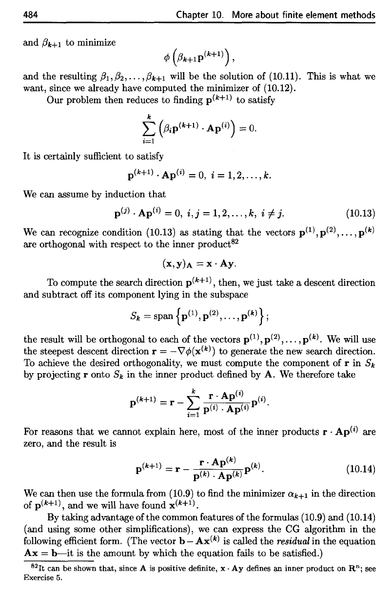
We
can recognize condition (10.13) as stating
that
the vectors
p(1),
p(2),
...
,
p(k)
are orthogonal with respect
to
the
inner product
82
(X,Y)A
= X·
Ay.
To compute
the
search direction
p(k+
I
),
then,
we
just take a descent direction
and subtract off its component lying in the subspace
Sk
= span
{p(1),
p(2),
...
,
p(k)
} ;
the result will be orthogonal
to
each of
the
vectors
p(1), p(2),
...
,p(k).
We
will use
the
steepest descent direction r =
-\7¢,(x(k))
to generate the new search direction.
To achieve the desired orthogonality,
we
must compute
the
component of r in
Sk
by projecting r onto
Sk
in
the
inner product defined by
A.
We
therefore take
(k+1) _ _
~
r·
Ap(i)
(i)
P - r
~
p(i)
.
Ap(i)
P .
•
=1
For reasons
that
we
cannot explain here, most of the inner products
r·
Ap(i)
are
zero,
and
the
result
is
(k+I)
_ _
r·
Ap(k)
(k)
P - r
p(k).
Ap(k)
P
(10.14)
We
can then use the formula from (10.9)
to
find the minimizer Ctk+1 in the direction
of
p(k+
I
) ,
and
we
will have found
x(k+
I
).
By taking advantage of
the
common features
ofthe
formulas (10.9) and (10.14)
(and using some other simplifications),
we
can express the CG algorithm in the
following efficient form. (The vector b -
Ax(k)
is called the residual in the equation
Ax
=
b-it
is
the
amount by which the equation fails to be satisfied.)
82It
can
be
shown
that,
since A is positive definite,
X·
Ay
defines
an
inner
product
on
Rnj
see
Exercise 5.
83
For
a
complete derivation
and
discussion
of the CG
algorithm,
see
[19],
for
example.
10.2.
Solving
sparse
linear
systems
485
The
reader should note
that
only
a
single
matrix-vector
product
is
required
at
each
step
of the
algorithm, making
it
very
efficient.
We
emphasize
that
we
have
not
derived
all of the
steps
in the CG
algorithm.
83
The
name "conjugate gradients"
is
derived
from
the
fact
that
many authors
refer
to the
orthogonality
of the
search directions,
in the
inner product
defined
by
A, as
A-conjugacy.
Therefore,
the key
step
is to
make
the
(negative) gradient
direction
conjugate
to the
previous search directions.
Example
10.3.
We
apply
100
steps
of
the CG
method
to the
system
Ku = f
from
Example
10.2.
The
result
differs
from
the
exact
solution
u by
about
0.001%
in the
Euclidean
norm,
and the
corresponding
piecewise
linear function
is
just
as
accurate
(error
of
about
3% in the
energy
norm)
as
that
obtained
from
solving
Ku
=
f
exactly.
10.2.6
Convergence
of the CG
algorithm
The CG
algorithm
was
constructed
so
that
the fcth
estimate,
x(
fc
),
of the
solution
x
minimizes
(j>
over
the fc-dimensional
subspace
Sk
=
spanjp^^p^
2
),...
,p^}.
Therefore,
x^
n
)
minimizes
0
over
an
n-dimensional
subspace
of
R
n
,
that
is,
over
all
of
R
n
.
It
follows
that
x(
n
)
must
be the
desired solution:
x(
n
)
= x.
Because
of
this observation,
the CG
algorithm
can be
regarded
as a
direct
method—it
computes
the
exact solution
after
a finite
number
of
steps
(at
least
when
performed
in floating
point arithmetic). There
are two
reasons, though,
why
this property
is
irrelevant:
1.
In floating
point arithmetic,
the
computed search directions
will
not
actually
be
A-conjugate (due
to the
accumulation
of
round-off
errors),
and so, in
fact,
x^
n
)
may
differ
significantly
from
x.
2.
Even
apart
from
the
issue
of
round-off
errors,
CG is not
used
as a
direct
method
for the
simple reason
that
n
steps
is too
many!
We
look
to
iterative
r = b
—
Ax (*
Compute
the
initial residual
*)
p
«—
r (*
Compute
the
initial search direction
*)
Ci
<-
r • r
for
fc =
l,2,...
v
«—
Ap
c
2
<-
p • v
o:
<—
^
(*
Solve
the
one-dimensional minimization problem
*)
x
-f-
x + ap (*
Update
the
estimate
of the
solution
*)
r
«—
r
—
CKV
(*
Compute
the new
residual
*)
c
3
«-
r • r
£<-S
p
-f-
ftp + r (*
Compute
the new
search direction
*)
Ci
<-C
3
10.2. Solving sparse linear systems
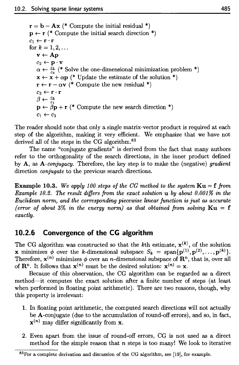
r = b -
Ax
(* Compute
the
initial residual *)
p +- r
(*
Compute
the
initial search direction
*)
Cl+-r·r
for k =
1,2,
...
v+-
Ap
C2+-P'V
0:
+-
~
(*
Solve
the
one-dimensional minimization problem *)
x +- x + o:p
(*
Update
the
estimate of
the
solution
*)
r +- r - o:v
(*
Compute
the
new residual
*)
c3+-
r
·
r
f3
+- ~
Cl
P +-
f3p
+ r
(*
Compute
the
new search direction
*)
Cl
+-
C3
485
The
reader should note
that
only a single matrix-vector product
is
required
at
each
step of
the
algorithm, making
it
very efficient.
We
emphasize
that
we
have
not
derived all
of
the
steps in
the
CG algorithm.
83
The
name "conjugate gradients" is derived from
the
fact
that
many
authors
refer
to
the
orthogonality of
the
search directions, in
the
inner product defined
by
A,
as
A-conjugacy.
Therefore,
the
key step is
to
make
the
(negative) gradient
direction conjugate
to
the
previous search directions.
Example
10.3.
We
apply 100 steps
of
the
CG
method
to the
system
Ku
= f from
Example 10.2. The result differs from the exact solution
u by about 0.001%
in
the
Euclidean
norm,
and
the corresponding piecewise linear
function
is
just
as accurate
(error
of
about
3%
in
the energy
norm)
as
that
obtained from solving
Ku
= f
exactly.
10.2.6 Convergence
of
the
CG
algorithm
The
CG algorithm was constructed so
that
the
kth
estimate,
x(k),
of
the
solution
x minimizes
4>
over
the
k-dimensional subspace
Sk
= span{p(1), p(2),
...
,p(k)}.
Therefore,
x(n)
minimizes
4>
over
an
n-dimensional subspace of Rn,
that
is, over all
of
Rn.
It
follows
that
x(n)
must be
the
desired solution:
x(n)
= x.
Because of this observation,
the
CG algorithm can be regarded as a direct
method-it
computes
the
exact solution after a finite number of steps
(at
least
when performed in floating point arithmetic). There are two reasons, though, why
this property is irrelevant:
1.
In
floating point arithmetic,
the
computed search directions will
not
actually
be A-conjugate (due
to
the
accumulation of round-off errors), and so, in fact,
x(n)
may differ significantly from x.
2.
Even
apart
from
the
issue of round-off errors, CG is
not
used as a direct
method for
the
simple reason
that
n steps is
too
many!
We
look
to
iterative
83For a complete derivation
and
discussion of
the
CG algorithm, see
[19],
for example.
2.
Suppose
A €
R
nxn
is
banded
with half-bandwidth
p.
Determine
the
exact
number
of
arithmetic operations required
to
factor
A
into
LU.
Exercises
1.
Suppose
A 6
R
nxn
.
Determine
the
exact number
of
arithmetic operations
required
for the
computation
of A = LU via
Gaussian elimination.
Further
count
the
number
of
operations required
to
compute
L
-1
b
and
U~
1
L~
1
b.
Verify
the
results given
in the
text.
The
following
formulas
will
be
useful:
486
Chapter
10.
More about
finite
element methods
methods when
n
is
very large, making Gaussian elimination
too
expensive.
In
such
a
case,
an
iterative method must give
a
reasonable approximation
in
much
less
than
n
iterations,
or it
also
is too
expensive.
The CG
algorithm
is
useful
precisely because
it can
give very good results
in a
relatively small
number
of
iterations.
The
rate
of
convergence
of CG is
related
to the
condition number
of A,
which
is
denned
as the
ratio
of the
largest eigenvalue
of A to the
smallest. When
the
condition number
is
relatively small
(that
is,
when
A is
well-conditioned),
CG
will
converge
rapidly.
The
algorithm also works
well
when
the
eigenvalues
of A are
clustered into
a few
groups.
In
this case, even
if the
largest eigenvalue
is
much
larger
than
the
smallest,
CG
will
perform
well.
The
worst case
for CG is a
matrix
A
whose eigenvalues
are
spread
out
over
a
wide range.
10.2.7
Preconditioned
CG
It is
often
possible
to
replace
a
matrix
A
with
a
related matrix whose eigenvalues
are
clustered,
and for
which
CG
will
converge quickly. This technique
is
called
preconditioning,
and it
requires
that
one find a
matrix
M
(the
preconditioned
that
is
somehow
similar
to A (in
terms
of its
eigenvalues)
but is
much simpler
to
invert.
At
each step
of the
preconditioned conjugate gradient (PCG) algorithm,
it is
necessary
to
solve
an
equation
of the
form
Mq = r.
Preconditioners
can be
found
in
many
different
ways,
but
most
require
an
intimate knowledge
of the
matrix
A. For
this reason, there
are few
general-purpose
methods.
One
method
that
is
often
used
is to
define
a
preconditioner
from
an
incomplete
factorization
of A. An
incomplete factorization
is a
factorization (like
Cholesky)
in
which
fill-in is
limited
by fiat.
Another method
for
constructing
pre-
conditioners
is to
replace
A by a
simpler matrix (perhaps arising
from
a
simpler
PDE)
that
can be
inverted
by FFT
methods.
486
Chapter 10. More
about
finite element methods
methods when n
is
very large, making Gaussian elimination too expensive.
In such a case, an iterative method must give a reasonable approximation in
much less
than
n iterations, or
it
also
is
too
expensive. The CG algorithm
is
useful precisely because it can give very good results in a relatively small
number of iterations.
The
rate
of convergence of CG
is
related to
the
condition number of A, which
is defined as the ratio of the largest eigenvalue of
A
to
the
smallest. When the
condition number
is
relatively small
(that
is, when A
is
well-conditioned), CG will
converge rapidly. The algorithm also works
well
when
the
eigenvalues of A are
clustered into a
few
groups. In this case, even if
the
largest eigenvalue
is
much
larger
than
the
smallest, CG will perform well. The worst case for CG
is
a matrix
A whose eigenvalues are spread out over a wide range.
10.2.7 Preconditioned
CG
It
is often possible
to
replace a matrix A with a related matrix whose eigenvalues
are clustered, and for which CG will converge quickly. This technique
is
called
preconditioning, and it requires
that
one find a matrix M (the preconditioner)
that
is
somehow similar
to
A (in terms of its eigenvalues)
but
is
much simpler to invert. At
each step of
the
preconditioned conjugate gradient (PCG) algorithm, it is necessary
to solve an equation of the form
Mq
=
r.
Preconditioners can be found in many different ways,
but
most require an
intimate knowledge of the matrix
A.
For this reason, there are
few
general-purpose
methods. One method
that
is often used
is
to define a preconditioner from an
incomplete factorization of
A.
An incomplete factorization
is
a factorization (like
Cholesky) in which fill-in is limited by fiat. Another method for constructing pre-
conditioners
is
to
replace A by a simpler matrix (perhaps arising from a simpler
PDE)
that
can be inverted by
FFT
methods.
Exercises
1. Suppose A E
Rnxn.
Determine the exact number of arithmetic operations
required for
the
computation of A =
LU
via Gaussian elimination. Further
count
the
number of operations required
to
compute
L-1b
and
U-1L-1b.
Verify the results given in the text. The following formulas will be useful:
ti =
n(n
+ 1),
i=l
2
ti
2
=
n(n+1)(2n+1).
i=l
6
2. Suppose A E
Rnxn
is banded with half-bandwidth p. Determine
the
exact
number of arithmetic operations required
to
factor A into L
U.
10.2.
Solving
sparse
linear
systems
487
3. Let A 6
R
nxn
be
symmetric,
and
suppose
b €
R
n
.
Define
(f>
as in
(10.7).
Show
that
(10.8) holds. (Hint:
One
method
is to
write
out
and
then show
that
Another method
is to
show
that
In
either case,
the
symmetry
of A is
essential.)
4.
Let A
e
R
nxn
be
SPD,
let
b,y
e
R
n
be
given,
and
suppose
a*
solves
where
Show
that
is
orthogonal
to
V0(y).
5.
Suppose
A e
R
nxn
is
SPD. Show
that
defines
an
inner product
on
R
n
.
6.
Let
{vi,
v
2
,...,
v
n
}
be a
linearly independent
set of
vectors
in an
inner prod-
uct
space,
and let G E
R
nxn
be the
corresponding Gram
matrix:
Prove
that
G is
SPD. (See
the
hint
for
Exercise 3.4.6.)
7.
The
quadratic
form
shown
in
Figures
10.10
and
10.11
is
where
10.2. Solving
sparse
linear systems
487
3.
Let A E Rnxn be symmetric, and suppose
bERn.
Define ¢ as in (10.7).
Show
that
(10.8) holds. (Hint: One method
is
to
write out
and then show
that
8¢
n
-8
(x) = "
AijXj
- bi ·
X·
L...J
Z
j=i
Another method
is
to
show
that
¢(x
+ y) = ¢(x) +
(Ax
-
b)
. y + 0
(1IYI12)
.
In either case, the symmetry of A
is
essential.)
4. Let A E Rnxn be SPD, let
b,y
E Rn be given, and suppose a* solves
where
Show
that
is
orthogonal to
V'
¢(y
).
min¢(y
- aV'¢(y)),
'"
1
¢(x)
=
-x·
Ax
- b . x.
2
V'¢(y - a*V'¢(y))
5.
Suppose A E Rnxn
is
SPD. Show
that
(X,y)A = X·
Ay
defines an inner product on R
n.
6.
Let
{Vi,
V2,
...
, v
n
}
be a linearly independent set of vectors in
an
inner prod-
uct space,
and
let G E Rnxn be the corresponding Gram matrix:
Prove
that
G
is
SPD. (See
the
hint for Exercise 3.4.6.)
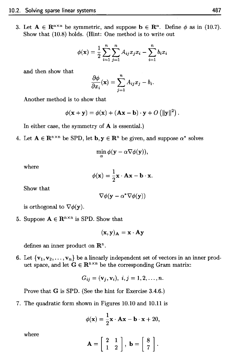
7.
The quadratic form shown in Figures 10.10 and 10.11
is
1
¢(x) =
2'x,
Ax
- b . x +
20,
where
A=[i
~],b=[~].