Gockenbach M.S. Partial Differential Equations. Analytical and Numerical Methods
Подождите немного. Документ загружается.

468
Chapter
10.
More
about
finite
element
methods
ElementList
1
2
3
4
5
6
7
8
9
10
11
12
13
14
15
16
17
18
19
20
21
22
23
24
25
26
27
28
29
30
31
32
1
1
2
2
6
2
7
3
7
7
8
8
389
3
4
4
6
6
7
7
8
8
9
9
11
11
12
12
13
13
14
14
16
16
17
17
18
18
19
19
4
9
5
11
7
12
8
13
9
14
10
16
12
17
13
18
14
19
15
21
17
22
18
23
19
24
20
9
10
10
12
12
13
13
14
14
15
15
17
17
18
18
19
19
20
20
22
22
23
23
24
24
25
25
NodeList
1
2
3
4
5
6
7
8
9
10
11
12
13
14
15
16
17
18
19
20
21
22
23
24
25
0
0.2500
0.5000
0.7500
1.0000
0
0.2500
0.5000
0.7500
1.0000
0
0.2500
0.5000
0.7500
1.0000
0
0.2500
0.5000
0.7500
1.0000
0
0.2500
0.5000
0.7500
1.0000
0
0
0
0
0
0.2500
0.2500
0.2500
0.2500
0.2500
0.5000
0.5000
0.5000
0.5000
0.5000
0.7500
0.7500
0.7500
0.7500
0.7500
1.0000
1.0000
1.0000
1.0000
1.0000
NodePtrs
1
2
3
4
5
6
7
8
9
10
11
12
13
14
15
16
17
18
19
20
21
22
23
24
25
0
0
0
0
0
0
1
2
3
0
0
4
5
6
0
0
7
8
9
0
0
0
0
0
0
PreeNodePtrs
1
2
3
4
5
6
7
8
9
7
8
9
12
13
14
17
18
19
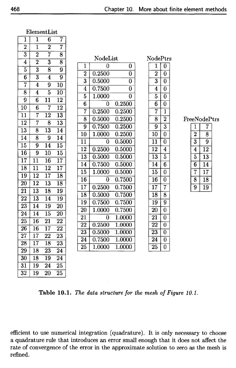
Table
10.1.
The
data
structure
for the
mesh
of
Figure
10.1.
efficient
to use
numerical integration
(quadrature).
It is
only necessary
to
choose
a
quadrature
rule
that
introduces
an
error small enough
that
it
does
not
affect
the
rate
of
convergence
of the
error
in the
approximate
solution
to
zero
as the
mesh
is
refined.
468
Chapter 10. More about finite element methods
ElementList
1 1
6 7
2 1 2
7
3 2
7 8
4 2
3 8
5
3 8 9
6 3
4
9
7
4
9 10
8
4
5
10
9 6
11
12
10
6
7
12
11
7
12 13
12
7
8
13
13
8
13 14
14
8 9
14
15
9
14 15
16 9 10 15
17
11
16 17
18
11
12 17
19 12 17 18
20
12
13
18
21
13 18
19
22
13 14 19
23
14 19 20
24 14
15 20
25
16
21
22
26
16
17
22
27
17
22 23
28
17
18 23
29
18
23
24
NodeList
1
0 0
2 0.2500
0
3
0.5000
0
4 0.7500
0
5
1.0000
0
6
0
0.2500
7 0.2500 0.2500
8
0.5000 0.2500
9
0.7500 0.2500
10 1.0000 0.2500
11
0
0.5000
12
0.2500 0.5000
13 0.5000 0.5000
14
0.7500
0.5000
15 1.0000 0.5000
16
0
0.7500
17
0.2500 0.7500
18 0.5000 0.7500
19
0.7500 0.7500
20
1.0000 0.7500
21
0
1.0000
22
0.2500 1.0000
23
0.5000
1.0000
24
0.7500 1.0000
25
1.0000 1.0000
NodePtrs
1
0
2
0
3
0
4
0
5 0
6 0
7
1
8
2
9
3
10 0
11
0
12
4
13
5
14
6
15
0
16
0
17
7
18
8
19
9
20
0
21
0
22
0
23
0
24
0
25
0
FreeN odePtrs
1
7
2
8
3 9
4
12
5
13
6
14
7 17
8 18
9
19
30 18 19 24
31
19
24 25
32 19 20
25
Table
10.1.
The data structure for the mesh
of
Figure 10.1.
efficient
to
use numerical integration (quadrature).
It
is only necessary
to
choose
a quadrature rule
that
introduces
an
error small enough
that
it does not affect the
rate
of convergence of
the
error in the approximate solution
to
zero as
the
mesh
is
refined.
A
quadrature rule
is an
approximation
of the
form
10.1.
Implementation
of
finite element methods
469
where
w\,
w?,...,
Wk,
the
weights,
are
real numbers
and
(si,
£1),
($2,
£2),...,
(fifc,
£&),
the
nodes,
are
points
in the
domain
of
integration
R.
Equation (10.1)
defines
a k
point quadrature rule.
Choosing
a
quadrature rule
There
are two
issues
that
must
be
resolved:
the
choice
of a
quadrature rule
and its
implementation
for an
arbitrary triangle.
We
begin
by
discussing
the
quadrature
rule.
A
useful
way to
classify
quadrature rules
is by
their
degree
of
precision. While
it may not be
completely obvious
at first, it is
possible
to
define
rules
of the
form
(10.1)
that
give
the
exact value when applied
to
certain polynomials.
A
rule
has
degree
of
precision
d if the
rule
is
exact
for all
polynomials
of
degree
d or
less. Since
both integration
and a
quadrature rule
of the
form
(10.1)
are
linear
in /, it
suffices
to
consider only monomials.
As
a
simple example, consider
the
rule
This
rule
has
degree
of
precision
1,
since
Equation (10.2)
is the
one-point Gaussian quadrature rule.
For
one-dimensional
integrals,
the
n-point
Gaussian quadrature rule
is
exact
for
polynomials
of
degree
2n
—
1 or
less.
For
example,
the
two-point Gauss quadrature rule, which
has
degree
of
precision
3, is
The
Gaussian quadrature rules
are
defined
on the
reference
interval
[-1,1];
to
apply
the
rules
on a
different
interval requires
a
simple change
of
variables.
In
multiple dimensions,
it is
also possible
to
define
quadrature rules with
a
given
degree
of
precision.
Of
course, things
are
more complicated because
of the
variety
of
geometries
that
are
possible.
We
will
exhibit rules
for
triangles with
degree
of
precision
1 and 2.
These rules
will
be
defined
for the
reference
triangle
10.1. Implementation of finite element methods
469
A quadrature rule
is
an approximation of
the
form
(10.1)
where
W1, W2,
...
,
Wk,
the
weights, are real numbers and (Sl' t1),
(S2'
t2),""
(Sk' tk),
the
nodes, are points in
the
domain of integration R. Equation (10.1) defines a k
point quadrature rule.
Choosing a quadrature rule
There are two issues
that
must be resolved:
the
choice of a quadrature rule
and
its
implementation for an arbitrary triangle.
We
begin by discussing the quadrature
rule. A useful way to classify quadrature rules
is
by their
degree
of
precision. While
it may not be completely obvious
at
first, it
is
possible
to
define rules of
the
form
(10.1)
that
give
the
exact value when applied to certain polynomials. A rule has
degree of precision
d if
the
rule
is
exact for all polynomials of degree d or less. Since
both
integration and a quadrature rule of the form (10.1) are linear in f, it suffices
to consider only monomials.
As
a simple example, consider
the
rule
[11
f(x)
dx
~
2f(0).
This rule has degree of precision
1,
since
p(x) = 1
::::}
[11
p(x) dx = 2 = 2p(0),
p(x)
= x::::}
[11
p(x) dx = 0 = 2p(0),
f1
2
p(x) = x
2
::::}
J
_/(x)
dx = 3
I=-
2p(O).
(10.2)
Equation (10.2)
is
the
one-point Gaussian quadrature rule. For one-dimensional
integrals,
the
n-point Gaussian quadrature rule
is
exact for polynomials of degree
2n
- 1 or less. For example, the two-point Gauss quadrature rule, which has degree
of precision
3,
is
The Gaussian quadrature rules are defined on the reference interval
[-1,
1];
to
apply
the rules on a different interval requires a simple change of variables.
In multiple dimensions, it
is
also possible to define quadrature rules with a
given degree of precision. Of course, things are more complicated because of
the
variety of geometries
that
are possible.
We
will exhibit rules for triangles with
degree of precision 1 and
2.
These rules will be defined for the reference triangle
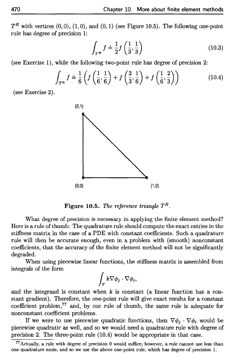
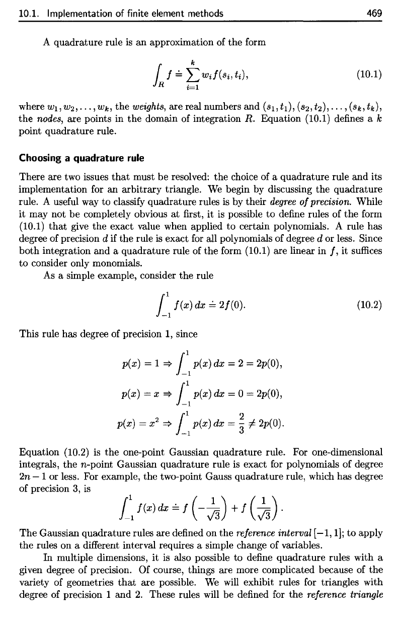
470
Chapter
10.
More about finite element methods
T
R
with vertices (0,0), (1,0),
and
(0,1)
(see Figure 10.5).
The
following
one-point
rule
has
degree
of
precision
1:
(see
Exercise
1),
while
the
following
two-point rule
has
degree
of
precision
2:
(see Exercise
2).
Figure
10.5.
The
reference
triangle
T
R
.
What degree
of
precision
is
necessary
in
applying
the finite
element method?
Here
is a
rule
of
thumb:
The
quadrature rule should compute
the
exact entries
in the
stiffness
matrix
in the
case
of a PDE
with constant
coefficients.
Such
a
quadrature
rule
will
then
be
accurate enough, even
in a
problem with (smooth)
nonconstant
coefficients,
that
the
accuracy
of the finite
element method
will
not be
significantly
degraded.
When using piecewise linear
functions,
the
stiffness
matrix
is
assembled
from
integrals
of the
form
and the
integrand
is
constant when
k is
constant
(a
linear
function
has a
con-
stant
gradient). Therefore,
the
one-point rule
will
give exact results
for a
constant
coefficient
problem,
77
and,
by our
rule
of
thumb,
the
same rule
is
adequate
for
nonconstant
coefficient
problems.
If
we
were
to use
piecewise quadratic
functions,
then
V0j
•
V0j
would
be
piecewise
quadratic
as
well,
and so we
would need
a
quadrature rule with degree
of
precision
2. The
three-point rule (10.4) would
be
appropriate
in
that
case.
77
Actually,
a
rule with degree
of
precision
0
would
suffice;
however,
a
rule cannot
use
less
than
one
quadrature
node,
and so we use the
above one-point rule, which
has
degree
of
precision
1.
470
Chapter
10.
More
about
finite
element
methods
TR
with vertices (0,0), (1,0), and (0,1) (see Figure 10.5). The following one-point
rule has degree of precision
1:
(10.3)
(see Exercise 1), while the following two-point rule has degree of precision
2:
(lOA)
(see Exercise 2).
(0,1)
(0,0)
(1,0)
Figure
10.5.
The reference triangle TR.
What
degree of precision
is
necessary in applying the finite element method?
Here
is
a rule of thumb: The quadrature rule should compute the exact entries in
the
stiffness matrix in the case of a PDE with constant coefficients. Such a quadrature
rule will then be accurate enough, even in a problem with (smooth) nonconstant
coefficients,
that
the accuracy of
the
finite element method will not be significantly
degraded.
When using piecewise linear functions,
the
stiffness matrix is assembled from
integrals of the form
L
k"VrPj
.
"VrPi,
and the integrand
is
constant when k
is
constant
(a
linear function has a con-
stant
gradient). Therefore,
the
one-point rule will give exact results for a constant
coefficient problem,77 and, by our rule of thumb,
the
same rule
is
adequate for
nonconstant coefficient problems.
If
we
were
to
use piecewise quadratic functions, then
"V
rPj
.
"V
rPi
would be
piecewise quadratic as well, and
so
we
would need a quadrature rule with degree of
precision
2.
The three-point rule
(lOA)
would be appropriate in
that
case.
77
Actually, a rule with degree of precision 0 would suffice; however, a rule cannot use less
than
one
quadrature
node,
and
so
we
use
the
above one-point rule, which has degree of precision 1.
10.1.
Implementation
of
finite
element methods
471
Integrating
over
an
arbitrary
triangle
There
is
still
the
following
technical
detail
to
discuss:
How can we
apply
a
quadra-
ture rule
defined
on the
reference
triangle
T
R
to an
integral over
an
arbitrary triangle
T? We
assume
that
T has
vertices
(pi,p2),
(tfi^),
and
(ri,r2).
We can
then
map
(^1,^2)
G
T
R
to
(xi,#2)
€
T by the
linear mapping
The
mapping (10.5) sends
(0,0),
(1,0),
and
(0,1)
to
(pi,p2),
(tfi,<?2),
and
(ri,r
2
),
respectively.
We
will
denote this mapping
by x =
F(y),
and we
note
that
the
Jacobian
matrix
of F is
We
can now
aonlv
the
rule
for a
change
of
variables
in a
multiple
integral:
78
As
the
determinant
of J is the
constant
it is
easy
to
apply
the
change
of
variables
and
then
any
desired quadrature rule.
For
example,
the
three-point rule (10.4)
would
be
applied
as
follows:
Exercises
1.
Verify
that
(10.3) produces
the
exact integral
for the
monomials
1, x, y.
2.
Verify
that
(10.4) produces
the
exact integral
for the
monomials
1, x,
?/,
x
2
,
xy,
y
2
.
3.
Let T be the
triangular region with vertices
(1,0),
(2,0),
and
(3/2,1),
and let
/ : T
->
R be
defined
by
/(x)
=
x\x\.
Compute
78
This
rule
is
explained
in
calculus texts such
as
Gillett [17],
or
more
fully
in
advanced calculus
texts
such
as
Kaplan
[29].
10.1. Implementation
of
finite element methods
471
Integrating over
an
arbitrary triangle
There is still
the
following technical detail
to
discuss: How can
we
apply a quadra-
ture
rule defined
on
the
reference triangle
TR
to
an
integral over
an
arbitrary
triangle
T? We assume
that
T has vertices (PI,P2), (ql,
q2),
and
(rl,
r2).
We
can
then
map
(ZI,Z2) E
TR
to
(XI,X2) E T by
the
linear mapping
Xl
= PI +
(ql
- pt}ZI +
(rl
-
PI)Z2,
X2
=
P2
+
(q2
-
P2)ZI
+
(r2
-
P2)Z2.
(10.5)
The
mapping (10.5) sends (0,0), (1,0),
and
(0,1)
to
(PI,P2), (ql,q2),
and
(rl,r2),
respectively. We will denote this mapping by x =
F(y),
and
we
note
that
the
Jacobian
matrix
of F
is
J = [
qi
- PI
rl
- PI ] .
q2
-
P2
r2
-
P2
We
can now apply
the
rule for a change of variables in a multiple integral:
78
r
f(x)dx=
{
f(F(y))ldet(J)1
dy.
iT
iTR
As
the
determinant of J is
the
constant
it
is easy
to
apply
the
change of variables
and
then
any desired
quadrature
rule.
For example,
the
three-point rule (10.4) would be applied as follows:
h f
==
I~I
(!
(X~l),
X~I))
+ f
(X~2)
,
X~2))
+ f
(X~3)
,
X~3)))
,
(X~I),
X~I))
=
(PI
+
(qi
-
PI)/6
+
(ri
- PI)/6,P2 +
(q2
- P2)/6 +
(r2
- P2)/6),
(x~2),
x~2))
=
(PI
+ 2(ql -
pt}/3
+
(ri
- PI)/6,P2 +
2(q2
- P2)/3 +
(r2
- P2)/6),
(X~3),
X~3))
=
(PI
+
(ql
-
pd/6
+
2(rl
- Pt}/3,P2 +
(q2
- P2)/6 +
2(r2
- P2)/3).
Exercises
1. Verify
that
(10.3) produces
the
exact integral for
the
monomials 1,
X,
y.
2.
Verify
that
(10.4) produces
the
exact integral for
the
monomials
1,
X,
y, x2,
xy,
y2.
3. Let T be
the
triangular region with vertices (1,0), (2,0), and
(3/2,1),
and
let
f : T -+ R
be
defined by
f(x)
=
XIX~.
Compute
78This rule is explained in calculus
texts
such as Gillett [17],
or
more fully in advanced calculus
texts
such as
Kaplan
[29].
472
Chapter
10.
More
about finite element methods
directly,
and
also
by
transforming
the
integral
to an
integral over
T
R
,
as
suggested
in the
text.
Verify
that
you
obtain
the
same result.
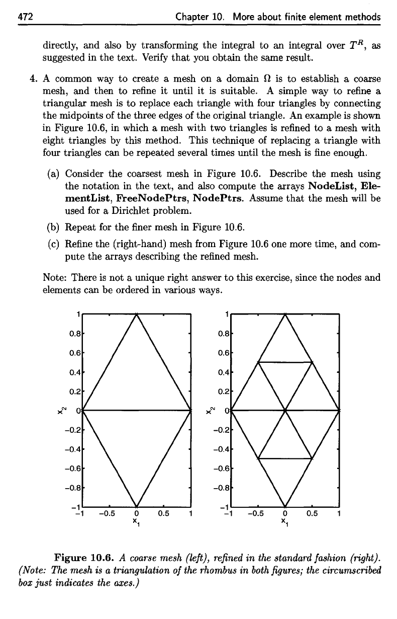
4.
A
common
way to
create
a
mesh
on a
domain
il
is to
establish
a
coarse
mesh,
and
then
to
refine
it
until
it is
suitable.
A
simple
way to
refine
a
triangular mesh
is to
replace each triangle with
four
triangles
by
connecting
the
midpoints
of the
three edges
of the
original triangle.
An
example
is
shown
in
Figure 10.6,
in
which
a
mesh with
two
triangles
is
refined
to a
mesh with
eight triangles
by
this method.
This
technique
of
replacing
a
triangle with
four
triangles
can be
repeated several times until
the
mesh
is fine
enough.
(a)
Consider
the
coarsest mesh
in
Figure 10.6. Describe
the
mesh using
the
notation
in the
text,
and
also compute
the
arrays
NodeList,
Ele-
mentList,
FreeNodePtrs,
NodePtrs.
Assume
that
the
mesh
will
be
used
for a
Dirichlet problem.
(b)
Repeat
for the finer
mesh
in
Figure 10.6.
(c)
Refine
the
(right-hand) mesh
from
Figure 10.6
one
more time,
and
com-
pute
the
arrays describing
the
refined
mesh.
Note:
There
is not a
unique right answer
to
this exercise, since
the
nodes
and
elements
can be
ordered
in
various ways.
Figure
10.6.
A
coarse
mesh
(left),
refined
in the
standard
fashion
(right).
(Note:
The
mesh
is a
triangulation
of
the
rhombus
in
both
figures; the
circumscribed
box
just
indicates
the
axes.)
472 Chapter 10. More about finite element methods
directly, and also by transforming the integral
to
an integral over
TR,
as
suggested in the text. Verify
that
you obtain the same result.
4.
A common way
to
create a mesh on a domain n
is
to establish a coarse
mesh, and then to refine it until
it
is
suitable. A simple way
to
refine a
triangular mesh
is
to
replace each triangle with four triangles by connecting
the
midpoints of the three edges of the original triangle. An example is shown
in Figure 10.6, in which a mesh with two triangles
is
refined
to
a mesh with
eight triangles by this method. This technique of replacing a triangle with
four triangles can be repeated several times until the mesh
is
fine enough.
(a) Consider the coarsest mesh in Figure 10.6. Describe the mesh using
the notation in the text, and also compute the arrays
NodeList,
Ele-
mentList,
FreeNodePtrs,
NodePtrs.
Assume
that
the mesh will be
used for a Dirichlet problem.
(b) Repeat
for
the finer mesh in Figure 10.6.
(c)
Refine the (right-hand) mesh from Figure 10.6 one more time, and com-
pute the arrays describing the refined mesh.
Note: There
is
not a unique right answer
to
this exercise, since the nodes and
elements can be ordered in various ways.
Figure
10.6.
A coarse mesh (left), refined in the standard fashion (right).
(Note: The mesh is a triangulation
of
the rhombus
in
both
figures; the circumscribed
box
just
indicates the axes.)
79
In
general, Gaussian elimination
is
numerically unstable unless partial pivoting
is
used.
Partial
pivoting
is the
technique
of
interchanging rows
to get the
largest possible pivot entry. This ensures
that
all of the
multipliers appearing
in the
algorithm
are
bounded above
by
one,
and in
virtually
every
case,
that
roundoff
error does
not
increase unduly. There
are
special classes
of
matrices,
most notably
the
class
of
symmetric positive
definite
matrices,
for
which
Gaussian elimination
is
provably
stable
with
no row
interchanges.
10.2.
Solving
sparse
linear systems
473
5.
Explain
how to use the
information stored
in the
data
structure suggested
in
the
text
to
solve
an
inhomogeneous Dirichlet problem.
6.
Consider
the
data
structure suggested
in the
text.
What information
is
lacking
that
is
needed
to
solve
an
inhomogeneous Neumann problem?
10.2 Solving
sparse
linear
systems
As
we
have mentioned several times,
the
finite
element method
is a
practical
nu-
merical method, even
for
large two-
and
three-dimensional problems, because
the
matrices
that
it
produces have mostly zero entries.
A
matrix
is
called
sparse
if a
large
percentage
of its
entries
are
known
to be
zero.
In
this
section,
we
wish
to
briefly
survey
the
subject
of
solving sparse linear systems.
Methods
for
solving linear systems
can be
divided into
two
categories.
A
method
that
will
produce
the
exact solution
in a
finite
number
of
steps
is
called
a
direct
method. (Actually, when implemented
on a
computer, even
a
direct method
will
not
compute
the
exact
solution because
of
unavoidable
round-off
error.
To be
precise,
a
direct method
will
compute
the
exact
solution
in a finite
number
of
steps,
provided
it is
implemented
in
exact arithmetic.)
The
most common direct methods
are
variants
of
Gaussian elimination. Below,
we
discuss modifications
of
Gaussian
elimination
for
sparse
matrices.
An
algorithm
that
computes
the
exact
solution
to a
linear system only
as
the
limit
of an
infinite
sequence
of
approximations
is
called
an
iterative method.
There
are
many iterative methods
in
use;
we
will
discuss
the
most popular:
the
conjugate
gradient algorithm.
We
also touch
on the
topic
of
preconditioning,
the
art of
transforming
a
linear system
so as to
obtain faster convergence with
an
iterative method.
10.2.1
Gaussian
elimination
for
dense
systems
In
order
to
have some
standard
of
comparison,
we first
briefly
discuss
the
standard
Gaussian elimination algorithm
for the
solution
of
dense systems.
Our
interest
is
in
the
operation
count—the
number
of
arithmetic operations necessary
to
solve
an
n
x
n
dense system.
The
basic algorithm
is
simple
to
write down.
In the
following
description,
we
assume
that
no row
interchanges
are
required,
as
these
do not use
any
arithmetic operations
anyway.
79
The
following
pseudo-code solves
Ax = b,
where
A €
R
nxn
and b
6
R
n
,
overwriting
the
values
of A and b:
10.2. Solving
sparse
linear systems
473
5.
Explain how to use the information stored in
the
data
structure suggested in
the
text
to
solve an inhomogeneous Dirichlet problem.
6.
Consider the
data
structure suggested in
the
text.
What
information is lacking
that
is needed to solve
an
inhomogeneous Neumann problem?
10.2 Solving sparse linear systems
As
we
have mentioned several times,
the
finite element method
is
a practical nu-
merical method, even for large two- and three-dimensional problems, because
the
matrices
that
it produces have mostly zero entries. A matrix
is
called sparse if a
large percentage of its entries are known
to
be zero. In this section,
we
wish
to
briefly survey the subject of solving sparse linear systems.
Methods for solving linear systems can be divided into two categories. A
method
that
will produce
the
exact solution in a finite number of steps
is
called a
direct method. (Actually, when implemented on a computer, even a direct method
will not compute
the
exact solution because of unavoidable round-off error. To be
precise, a direct method will compute
the
exact solution in a finite number of steps,
provided it
is
implemented in exact arithmetic.) The most common direct methods
are variants of Gaussian elimination. Below,
we
discuss modifications of Gaussian
elimination for sparse matrices.
An algorithm
that
computes the exact solution to a linear system only as
the
limit of
an
infinite sequence of approximations
is
called an iterative method.
There are many iterative methods in use;
we
will discuss the most popular:
the
conjugate gradient algorithm.
We
also touch on
the
topic of preconditioning, the
art
of transforming a linear system
so
as
to
obtain faster convergence with an
iterative method.
10.2.1
Gaussian
elimination for
dense
systems
In order
to
have some standard of comparison,
we
first briefly discuss the standard
Gaussian elimination algorithm for the solution of dense systems. Our interest
is
in
the
operation
count-the
number of arithmetic operations necessary to solve
an
n x n dense system. The basic algorithm
is
simple
to
write down. In
the
following
description,
we
assume
that
no row interchanges are required, as these do not use
any arithmetic operations anyway.
79
The following pseudo-code solves
Ax
=
b,
where A E
Rnxn
and
bERn,
overwriting the values of A and
b:
for i = 1,2,
...
, n - 1
for
j = i +
1,
i + 2,
...
, n
k·
t-
~
______
3'_
Aii
79In general, Gaussian elimination is numerically unstable unless partial pivoting is used.
Partial
pivoting is
the
technique of interchanging rows
to
get
the
largest possible pivot entry.
This
ensures
that
all of
the
multipliers appearing in
the
algorithm are
bounded
above by one,
and
in virtually
every case,
that
roundoff error does
not
increase unduly.
There
are
special classes of matrices,
most notably
the
class of symmetric positive definite matrices, for which Gaussian elimination is
provably stable with no row interchanges.
474
Chapter
10.
More about
finite
element methods
The first
(nested) loop
is
properly called Gaussian elimination;
it
systemati-
cally
eliminates variables
to
produce
an
upper triangular system
that
is
equivalent
to the
original system.
The
second loop
is
called
back
substitution;
it
solves
the
last equation, which
now has
only
one
variable,
for
#
n
,
substitutes
this
value
in
the
preceding equation
and
solves
for
or
n
_i,
and so
forth.
The
pseudo-code above
overwrites
the
right-hand-side vector
b
with
the
solution
x.
The
Gaussian elimination
part
of the
algorithm
is
equivalent (when,
as we
have
assumed,
no row
interchanges
are
required)
to
factoring
A
into
the
product
of
an
upper triangular matrix
U and a
unit lower triangular matrix
(that
is, a
lower
triangular matrix with
all
ones
on the
diagonal)
L: A = LU. As the
algorithm
is
written above,
the
matrix
A is
overwritten with
the
value
of U (on and
above
the
diagonal)
and L
(below
the
diagonal—there
is no
need
to
store
the
diagonal
of
L,
since
it is
known
to
consist
of all
ones).
At the
same time,
the first
loop above
effectively
replaces
b by
L
-1
b.
The
back substitution phase
is
then equivalent
to
replacing
L~
x
b
by
U~
1
L~
1
b
=
A
-1
b.
The
factorization
A = LU is
simply called
the LU
factorization.
It is not
difficult
to
count
the
number
of
arithmetic
operations
required
by
Gaussian elimination
and
back substitution.
It
turns
out to be
with most
of the
operations
used
to
factor
A
into
LU
(the
computation
of L
x
b
and
then
U~
1
L~
1
b
requires only
O(2n
2
)
operations). (Exercise
1
asks
the
reader
to
verify
these results.)
When
the
matrix
A is
symmetric
and
positive
definite
80
(SPD),
then
one can
take
advantage
of
symmetry
to
factor
the
matrix
as A =
LL
T
,
where
L is
lower
triangular.
This
factorization
is
called
the
Cholesky
factorization. (The Cholesky
factor
L is not the
same matrix
L
appearing
in the LU
factorization—in
particular,
it
does
not
have
all
ones
on the
diagonal—but
it is
closely related.)
The
symmetry
of
A
makes
the
Cholesky factorization less expensive
than
the LU
factorization;
the
operation count
is
O(n
3
/3).
For
simplicity (because
the
Cholesky factorization
is
less familiar
and
harder
to
describe
than
the LU
factorization),
we
will discuss
the
direct solution
of
linear systems
in
terms
of
Gaussian elimination
and the LU
factorization. However,
the
reader should bear
in
mind
that
the
stiffness
matrix
K
is
SPD,
and so the
Cholesky factorization
is
preferred
in
practice.
80
The
reader should recall that
a
symmetric matrix
A
e
R
nXn
is
called positive
definite
if
x
G
R
n
,
x
^
0
=»
x • Ax > 0.
The
matrix
A is
positive
definite
if and
only
if all of its
eigenvalues
are
positive.
474
b
j
+-
bj -
Ajibi
for k = i +
1,
i +
2,
...
, n
Ajk
+-
Ajk
-
AjiAik
for i =
n,
n - 1,
...
,1
Chapter
10.
More about finite element methods
b
i
+-
(b
i
-
E7=i+1
Aijb
j
)
/Aii
The first (nested) loop
is
properly called Gaussian elimination; it systemati-
cally eliminates variables to produce
an
upper triangular system
that
is
equivalent
to
the
original system. The second loop
is
called back substitution; it solves the
last equation, which now has only one variable, for
X
n
,
substitutes this value in
the
preceding equation and solves for X
n
-1,
and so forth. The pseudo-code above
overwrites
the
right-hand-side vector b with the solution x.
The Gaussian elimination
part
of
the
algorithm
is
equivalent (when, as
we
have assumed, no row interchanges are required)
to
factoring A into
the
product of
an upper triangular matrix U and a
unit
lower triangular matrix
(that
is, a lower
triangular matrix with all ones on the diagonal)
L:
A =
LU.
As
the algorithm
is
written above,
the
matrix A
is
overwritten with
the
value of U (on and above
the
diagonal) and L (below
the
diagonal-there
is
no need
to
store the diagonal of
L, since
it
is
known
to
consist of all ones). At the same time, the first loop above
effectively replaces b by L
-1
b.
The back substitution phase
is
then equivalent
to
replacing
L-
1
b
by
U-1L-
1
b
= A
-lb.
The
factorization A =
LU
is simply called
the
LU
factorization.
It
is
not difficult to count
the
number of arithmetic operations required by
Gaussian elimination
and
back substitution.
It
turns out
to
be
with most of the operations used
to
factor A into L U (the computation of L
-1
b
and
then
U-
1
L
-1
b requires only O(2n2) operations). (Exercise 1 asks the reader
to
verify these results.)
When the matrix A is symmetric
and
positive definite
80
(SPD), then one can
take advantage of symmetry
to
factor
the
matrix as A =
LL
T
,
where L
is
lower
triangular. This factorization is called
the
Cholesky factorization. (The Cholesky
factor L
is
not
the
same matrix L appearing in
the
LU
factorization-in
particular,
it
does not have all ones on
the
diagonal-but
it is closely related.) The symmetry
of
A makes the Cholesky factorization less expensive
than
the
LU
factorization;
the
operation count
is
O(n
3
/3). For simplicity (because
the
Cholesky factorization
is less familiar and harder
to
describe
than
the LU factorization),
we
will discuss
the
direct solution of linear systems in terms of Gaussian elimination and the
LU
factorization. However, the reader should bear in mind
that
the
stiffness matrix K
is
SPD, and
so
the
Cholesky factorization is preferred in practice.
80
The
reader
should recall
that
a
symmetric
matrix
A E
Rnxn
is called positive definite if
xER
n
,
x,tO=}x·Ax>O.
The
matrix
A is positive definite
if
and
only if all
of
its
eigenvalues are positive.
10.2.
Solving
sparse linear systems
475
n
100
200
400
800
1600
time
(s)
0.0116
0.107
1.57
12.7
102
Table 10.2.
personal
computer.
Time
required
to
solve
an n x n
dense
linear system
on a
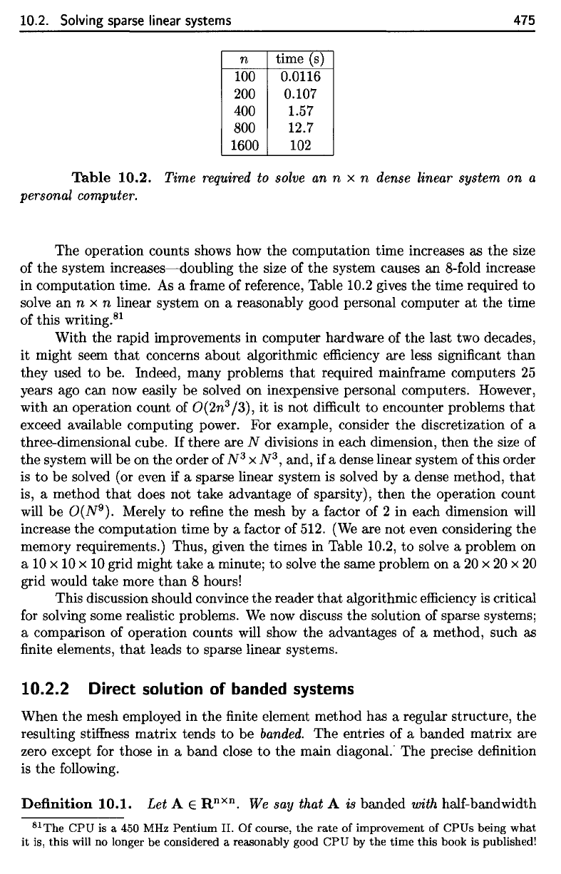
The
operation counts shows
how the
computation time increases
as the
size
of
the
system
increases—doubling
the
size
of the
system causes
an
8-fold
increase
in
computation time.
As a
frame
of
reference, Table 10.2 gives
the
time required
to
solve
an n x n
linear system
on a
reasonably good personal computer
at the
time
of
this
writing.
81
With
the
rapid improvements
in
computer hardware
of the
last
two
decades,
it
might seem
that
concerns about algorithmic
efficiency
are
less significant
than
they used
to be.
Indeed, many problems
that
required mainframe computers
25
years
ago can now
easily
be
solved
on
inexpensive personal computers. However,
with
an
operation count
of
0(2n
3
/3),
it is not
difficult
to
encounter problems
that
exceed
available computing power.
For
example, consider
the
discretization
of a
three-dimensional cube.
If
there
are N
divisions
in
each dimension, then
the
size
of
the
system
will
be on the
order
of
N
3
x
N
3
,
and,
if a
dense linear system
of
this order
is
to be
solved
(or
even
if a
sparse linear system
is
solved
by a
dense method,
that
is,
a
method
that
does
not
take advantage
of
sparsity), then
the
operation count
will
be
O(N
9
).
Merely
to
refine
the
mesh
by a
factor
of 2 in
each dimension
will
increase
the
computation time
by a
factor
of
512.
(We are not
even considering
the
memory
requirements.) Thus, given
the
times
in
Table 10.2,
to
solve
a
problem
on
a 10 x 10 x 10
grid might
take
a
minute;
to
solve
the
same problem
on a 20 x 20 x 20
grid would take more
than
8
hours!
This discussion should convince
the
reader
that
algorithmic
efficiency
is
critical
for
solving some realistic problems.
We now
discuss
the
solution
of
sparse systems;
a
comparison
of
operation counts
will
show
the
advantages
of a
method, such
as
finite
elements,
that
leads
to
sparse linear systems.
10.2.2
Direct
solution
of
banded systems
When
the
mesh employed
in the finite
element method
has a
regular structure,
the
resulting
stiffness
matrix tends
to be
banded.
The
entries
of a
banded matrix
are
zero
except
for
those
in a
band close
to the
main
diagonal.
The
precise
definition
is
the
following.
Definition 10.1.
Let A
e
R
nxn
.
We
say
that
A is
banded with half-bandwidth
81
The CPU is a 450 MHz
Pentium
II. Of
course,
the
rate
of
improvement
of
CPUs being what
it
is,
this will
no
longer
be
considered
a
reasonably good
CPU by the
time this book
is
published!
10.2. Solving sparse linear systems
475
n
time (s)
100
0.0116
200
0.107
400 1.57
800
12.7
1600
102
Table
10.2.
Time required to solve an n x n dense linear system on a
personal computer.
The operation counts shows how
the
computation time increases as the size
of
the
system increases--doubling
the
size of the system causes an 8-fold increase
in computation time.
As
a frame of reference, Table 10.2 gives
the
time required
to
solve
an
n x n linear system on a reasonably good personal computer
at
the
time
of this writing.
81
With the rapid improvements in computer hardware of
the
last two decades,
it
might seem
that
concerns about algorithmic efficiency are less significant
than
they used
to
be. Indeed, many problems
that
required mainframe computers
25
years ago can now easily be solved on inexpensive personal computers. However,
with
an
operation count of
O(2
n
3/3), it
is
not difficult to encounter problems
that
exceed available computing power. For example, consider
the
discretization of a
three-dimensional cube.
If
there are N divisions in each dimension, then the size of
the
system will be on the order of
N3
x
N3,
and, if a dense linear system of this order
is
to
be solved (or even if a sparse linear system
is
solved by a dense method,
that
is, a method
that
does not take advantage of sparsity), then
the
operation count
will be
O(N9). Merely to refine the mesh by a factor of 2 in each dimension will
increase the computation time by a factor of 512. (We are not even considering the
memory requirements.) Thus, given the times in Table 10.2,
to
solve a problem on
a
10
x
10
x
10
grid might take a minute;
to
solve the same problem on a
20
x
20
x
20
grid would take more
than
8 hours!
This discussion should convince the reader
that
algorithmic efficiency
is
critical
for solving some realistic problems.
We
now discuss the solution of sparse systems;
a comparison of operation counts will show the advantages of a method, such as
finite elements,
that
leads to sparse linear systems.
10.2.2 Direct solution
of
banded systems
When
the
mesh employed in the finite element method has a regular structure,
the
resulting stiffness matrix tends
to
be
banded.
The
entries of a banded matrix are
zero except for those in a band close
to
the
main diagonal: The precise definition
is
the following.
Definition
10.1.
Let A E
Rnxn.
We say that A is banded with half-bandwidth
81The
CPU
is a 450 MHz
Pentium
II.
Of
course,
the
rate
of
improvement
of
CPUs
being
what
it
is, this will no longer be considered a reasonably good
CPU
by
the
time
this
book is published!
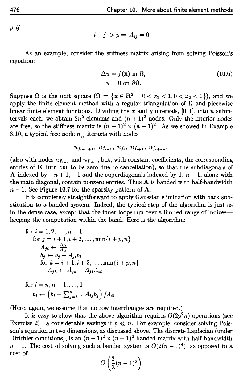
476
Chapter
10.
More about
finite
element methods
P
if
As an
example, consider
the
stiffness
matrix arising
from
solving
Poisson's
equation:
Suppose
£7 is the
unit square
(J7
= {x € R
2
: 0 <
x\
< 1,0 <
#2
<
l})>
and we
apply
the finite
element method with
a
regular
triangulation
of
f)
and
piecewise
linear
finite
element
functions.
Dividing
the x and y
intervals,
[0,1],
into
n
subin-
tervals each,
we
obtain
2n
2
elements
and (n +
I)
2
nodes. Only
the
interior nodes
are
free,
so the
stiffness
matrix
is (n —
I)
2
x (n —
I)
2
.
As we
showed
in
Example
8.10,
a
typical
free
node
rif
i
iteracts
with nodes
(also with nodes
n/
i-n
and
n/
i+n
,
but, with constant
coefficients,
the
corresponding
entries
of K
turn
out to be
zero
due to
cancellation),
so
that
the
subdiagonals
of
A
indexed
by
—
n + 1,
—
1 and the
superdiagonals indexed
by
1,
n
—
1,
along with
the
main diagonal, contain nonzero entries. Thus
A is
banded with half-bandwidth
n - 1. See
Figure 10.7
for
the
sparsity
pattern
of A.
It is
completely straightforward
to
apply Gaussian elimination with back sub-
stitution
to a
banded system. Indeed,
the
typical step
of the
algorithm
is
just
as
in
the
dense case, except
that
the
inner loops
run
over
a
limited range
of
indices—
keeping
the
computation within
the
band.
Here
is the
algorithm:
(Here,
again,
we
assume
that
no row
interchanges
are
required.)
It is
easy
to
show
that
the
above algorithm requires
O(2p
2
n)
operations (see
Exercise
2)—a
considerable savings
if p
<£
n. For
example, consider solving
Pois-
son's equation
in two
dimensions,
as
discussed above.
The
discrete
Laplacian
(under
Dirichlet conditions),
is an (n
—
I)
2
x (n
—
I)
2
banded matrix with half-bandwidth
n
—
1.
The
cost
of
solving such
a
banded system
is
O(2(n
—
I)
4
),
as
opposed
to a
cost
of
476
Chapter 10.
More
about finite element methods
p
if
li-jl
>p=>A
ij
=0.
As
an
example, consider the stiffness matrix arising from solving Poisson's
equation:
-~u
=
f(x)
in
n,
u = 0 on
an.
(10.6)
Suppose n
is
the
unit square
(n
=
{x
E
R2
: 0 <
Xl
<
1,0
< X2 <
I}),
and
we
apply
the
finite element method with a regular triangulation of n and piecewise
linear finite element functions. Dividing
the
X and y intervals, [0,1], into n subin-
tervals each,
we
obtain
2n
2
elements
and
(n
+
1)2
nodes. Only the interior nodes
are free, so
the
stiffness matrix
is
(n -
1)
2 X (n - 1)2.
As
we
showed in Example
8.10, a typical free node
n/;
iteracts with nodes
(also with nodes
n
/;-n
and n
/;+n'
but, with constant coefficients, the corresponding
entries of K
turn
out
to
be zero due
to
cancellation), so
that
the sub diagonals of
A indexed by
-n
+
1,
-1
and the superdiagonals indexed by
1,
n -
1,
along with
the
main diagonal, contain nonzero entries. Thus A
is
banded with half-bandwidth
n - 1. See Figure 10.7 for the sparsity
pattern
of
A.
It
is
completely straightforward
to
apply Gaussian elimination with back sub-
stitution
to
a banded system. Indeed, the typical step of the algorithm
is
just
as
in
the
dense case, except
that
the inner loops
run
over a limited range of
indices-
keeping the computation within the band. Here
is
the algorithm:
for i
= 1,2,
...
, n - 1
for
j = i +
1,
i +
2,
...
,
mini
i + p, n}
k·
t-
~
J~
Ai;
b
j
t-
b
j
-
Ajibi
for k = i +
1,i
+
2,
...
,min{i +
p,n}
Ajk
t-
Ajk
-
AjiAik
for i = n, n -
1,
...
,1
bi
t-
(b
i -
Ej=i+l
Aijb
j
)
jAii
(Here, again,
we
assume
that
no row interchanges are required.)
It
is easy
to
show
that
the
above algorithm requires O(2p
2
n) operations (see
Exercise
2)-a
considerable savings
if
p
«n.
For example, consider solving Pois-
son's equation in two dimensions, as discussed above. The discrete Laplacian (under
Dirichlet conditions),
is
an
(n -
1)2
x (n -
1)2
banded matrix with half-bandwidth
n - 1. The cost of solving such a banded system
is
O(2(n - 1)4), as opposed
to
a
cost of
10.2.
Solving
sparse
linear systems
477
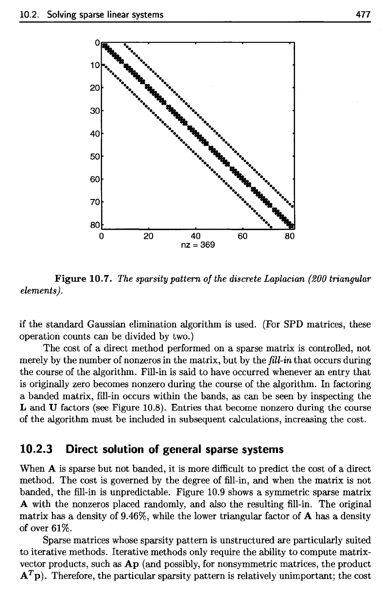
Figure
10.7.
The
sparsity
pattern
of
the
discrete
Laplacian
(200 triangular
elements).
if
the
standard
Gaussian
elimination algorithm
is
used.
(For
SPD
matrices,
these
operation counts
can be
divided
by
two.)
The
cost
of a
direct method
performed
on a
sparse matrix
is
controlled,
not
merely
by the
number
of
nonzeros
in the
matrix,
but by the fill-in
that
occurs during
the
course
of the
algorithm. Fill-in
is
said
to
have occurred whenever
an
entry
that
is
originally zero becomes nonzero during
the
course
of the
algorithm.
In
factoring
a
banded matrix,
fill-in
occurs within
the
bands,
as can be
seen
by
inspecting
the
L
and U
factors
(see
Figure 10.8). Entries
that
become nonzero during
the
course
of
the
algorithm must
be
included
in
subsequent calculations, increasing
the
cost.
10.2.3
Direct
solution
of
general
sparse systems
When
A is
sparse
but not
banded,
it is
more
difficult
to
predict
the
cost
of a
direct
method.
The
cost
is
governed
by the
degree
of fill-in, and
when
the
matrix
is not
banded,
the fill-in is
unpredictable. Figure
10.9
shows
a
symmetric sparse matrix
A
with
the
nonzeros placed randomly,
and
also
the
resulting
fill-in. The
original
matrix
has a
density
of
9.46%,
while
the
lower
triangular factor
of A has a
density
of
over 61%.
Sparse matrices whose sparsity pattern
is
unstructured
are
particularly suited
to
iterative methods. Iterative methods only require
the
ability
to
compute matrix-
vector products, such
as Ap
(and
possibly,
for
nonsymmetric matrices,
the
product
A
T
p).
Therefore,
the
particular sparsity
pattern
is
relatively unimportant;
the
cost
10.2. Solving sparse linear systems
..
••
..
10
_.
,
••••••
_.
e.
-.
-.
20
••••
,
••••
e.
_.
_.
e.
.....•
,
..••..
-. -.
.•...
,
...•.
-.
-.
-. -.
-.
-.
..•...
,
•..•..
_.
e.
....
,
....
e.
_.
-. -.
-.
-.
30
40
50
60
-.
-.
...
,
...
-.
-.
-.
-.
-.
-.
70
..
..
••
80~
______
~
______
~
_____________
~~.
__
~
o
20
40
60 80
nz
= 369
477
Figure
10.7.
The sparsity pattern
of
the discrete Laplacian (200 triangular
elements).
if
the
standard
Gaussian elimination algorithm is used. (For SPD matrices, these
operation counts can be divided by two.)
The cost of a direct method performed on a sparse matrix
is
controlled, not
merely by
the
number of nonzeros in the matrix,
but
by the fill-in
that
occurs during
the
course of the algorithm. Fill-in
is
said
to
have occurred whenever an entry
that
is
originally zero becomes nonzero during the course of the algorithm. In factoring
a banded matrix, fill-in occurs within
the
bands, as can be seen by inspecting
the
Land
U factors (see Figure 10.8). Entries
that
become nonzero during the course
of
the
algorithm must be included in subsequent calculations, increasing the cost.
10.2.3 Direct solution of general
sparse
systems
When A
is
sparse
but
not banded, it
is
more difficult
to
predict the cost of a direct
method. The cost
is
governed by the degree of fill-in, and when
the
matrix is not
banded, the fill-in is unpredictable. Figure 10.9 shows a symmetric sparse matrix
A with the nonzeros placed randomly, and also the resulting fill-in.
The
original
matrix has a density of 9.46%, while the lower triangular factor of A has a density
of over 61%.
Sparse matrices whose sparsity
pattern
is
unstructured are particularly suited
to
iterative methods. Iterative methods only require the ability
to
compute matrix-
vector products, such as
Ap
(and possibly, for nonsymmetric matrices,
the
product
AT
p).
Therefore, the particular sparsity
pattern
is
relatively unimportant; the cost