Gockenbach M.S. Partial Differential Equations. Analytical and Numerical Methods

458

Chapter

9.

More about Fourier

series

IB VP

The

question

we

wish

to

answer

is:

What

is the

lowest frequency

at

which

the

membrane will resonate? This

could

be an

important consideration

in

designing

a

device

that contained such

a

membrane.

The key

point

is

that,

if

we

knew

the

eigenvalues

and

eigenvectors

of

the

nega-

tive Laplacian

on fi

(subject

to

Dirichlet conditions), then

we

could

solve

the

IBVP

just

as in the

Fourier series method. Suppose

the

eigenpairs

are

Then

we can

write

the

solution

w(x,£)

as

Substituting into

the PDE

yields

and

so

a

n

(t)

satisfies

Therefore,

with

the

coefficients

b

n

and

c

n

determined

by the

initial conditions.

Therefore,

the

fundamental

frequency—the

smallest natural

frequency—of

the

membrane

is

cx/V^TT).

This

example

shows

that

we

would

gain

some useful information

by

computing

the

smallest eigenvalue

of the

operator

on

£).

We

will revisit

this

example

in

Section

10.4, where

we use finite

element methods

to

estimate

the

smallest eigenvalue

of

various domains.

Exercises

1.

Prove

that

the

operator

K

defined above

is

symmetric.

458

Chapter

9.

More about Fourier series

IBVP

a

2

u 2

at

2

-

c

Au

= 0, x E

n,

t > 0,

u(x,O) = ¢(x), x E

n,

au

at (x,O) = ,),(x), x E

n,

u(x,

t) = 0, x E

an,

t >

O.

(9.28)

The question

we

wish to answer is: What is the lowest frequency

at

which the

membrane will resonate? This could

be

an important consideration in designing a

device that contained such a membrane.

The key point is that,

if

we

knew the eigenvalues and eigenvectors

of

the nega-

tive Laplacian on

n (subject to Dirichlet conditions), then

we

could solve the

IBVP

just

as

in the Fourier series method. Suppose the eigenpairs

are

An,

'l/Jn(x)

, n =

1,2,3,

....

Then

we

can write the solution

u(x,

t)

as

00

u(x,

t) =

l:

an (t)'l/Jn(x).

n=l

Substituting into the

PDE

yields

and

so

an(t) satisfies

Therefore,

an(t)

= b

n

cos

(cAt)

+ C

n

sin

(cAt),

with the coefficients b

n

and

en

determined

by

the initial conditions. Therefore,

the fundamental

frequency-the

smallest natural

frequency-of

the membrane is

cv'):; / (2n).

This example shows

that

we would gain some useful information by computing

the

smallest eigenvalue of

the

operator

on

n.

We

will revisit this example

in

Section

lOA, where

we

use finite element methods

to

estimate

the

smallest eigenvalue

of

various domains.

Exercises

1. Prove

that

the

operator

K defined above is symmetric.

9.8.

Suggestions

for

further reading

The books cited in Section 5.8 as dealing with Fourier series all present the con-

vergence theory. More specialized books, both with a wealth of information about

Fourier series and other aspects of Fourier analysis, are Kammler

[28)

and Folland

[15].

Folland's book

is

classical in nature, while Kammler delves into a number of

applications of modern interest.

Briggs and Henson

[7]

gives a comprehensive introduction

to

the discrete

Fourier transform and covers some applications, while Van Loan

[50)

provides an

in-depth treatment of the mathematics of

the

fast Fourier transform. Other texts

that

explain the

FFT

algorithm include Walker

[51]

and

Brigham

[8].

This page intentionally left blank

Chapter

10

More

about finite element

In

this chapter,

we

will

look more deeply into

finite

element methods

for

solving

steady-state

BVPs.

Finite

element methods

form

a

vast

area,

and

even

by the end

of

this chapter,

we

will

have only scratched

the

surface.

Our

goal

is

modest:

We

wish

to

give

the

reader

a

better

idea

of how

finite

element methods

are

implemented

in

practice,

and

also

to

give

an

overview

of the

convergence theory.

The

main

tasks

involved

in

applying

the

finite

element method

are

•

Defining

a

mesh

on the

computational domain.

•

Computing

the

stiffness

matrix

K and the

load vector

f.

•

Solving

the

finite

element equation

Ku =

f.

We

will

mostly ignore

the first

question, except

to

provide examples

for

simple

do-

mains. Mesh generation

is an

area

of

study

in its own

right,

and

delving into

this

subject

is

beyond

the

scope

of

this book.

We

begin

by

addressing issues involved

in

computing

the

stiffness

matrix

and

load vector, including

data

structures

for

representing

and

manipulating

the

mesh.

We

will concentrate

on

two-dimensional

problems, triangular meshes,

and

piecewise linear

finite

elements,

as

these

are

suf-

ficient to

illustrate

the

main ideas. Next,

in

Section 10.2,

we

discuss methods

for

solving

the finite

element equation

Ku =

f,

specifically,

on

algorithms

for

taking

advantage

of the

sparsity

of

this system

of

equations.

In

Section 10.3,

we

provide

a

brief

outline

of the

convergence theory

for

Galerkin

finite

element methods. Finally,

we

close

the

book with

a

discussion

of finite

element methods

for

solving eigenvalue

problems, such

as

those suggested

in

Section 9.7.

10.1

Implementation

of

finite

element methods

There

are

several issues

that

must

be

resolved

in

order

to

efficiently

implement

the

finite

element method

in a

computer program, including

•

Data

structures

for

representation

of the

mesh.

461

methods

Chapter 10

about finite element

In this chapter,

we

will look more deeply into finite element methods for solving

steady-state BVPs. Finite element methods form a vast area, and even by the end

of this chapter,

we

will have only scratched the surface. Our goal

is

modest:

We

wish

to

give the reader a

better

idea of how finite element methods are implemented

in practice, and also

to

give

an

overview of the convergence theory.

The main tasks involved in applying the finite element method are

• Defining a mesh on

the

computational domain.

• Computing the stiffness matrix K and the load vector

f.

• Solving the finite element equation

Ku

=

f.

We

will mostly ignore

the

first question, except to provide examples for simple do-

mains. Mesh generation

is

an area of study in its own right, and delving into this

subject

is

beyond the scope of this book.

We

begin by addressing issues involved

in computing the stiffness matrix

and

load vector, including

data

structures for

representing and manipulating the mesh.

We

will concentrate on two-dimensional

problems, triangular meshes,

and

piecewise linear finite elements, as these are suf-

ficient

to

illustrate

the

main ideas. Next, in Section 10.2,

we

discuss methods for

solving

the

finite element equation

Ku

= f, specifically, on algorithms for taking

advantage of

the

sparsity of this system of equations. In Section 10.3,

we

provide a

brief outline of

the

convergence theory for Galerkin finite element methods. Finally,

we

close

the

book with a discussion of finite element methods for solving eigenvalue

problems, such as those suggested in Section 9.7.

10.1 Implementation

of

finite element methods

There are several issues

that

must be resolved in order to efficiently implement the

finite element method in a computer program, including

•

Data

structures for representation of the mesh.

461

462

Chapter

10.

More about

finite

element methods

•

Efficient

computation

of the

various integrals

that

define

the

entries

in the

stiffness

matrix

and

load vector.

•

Algorithms

for

assembling

the

stiffness

matrix

and the

load vector.

We

will

now

discuss these issues.

10.1.1

Describing

a

triangulation

Before

we can

describe

data

structures

and

algorithms,

we

must develop

notation

for

the

computational mesh. First

of

all,

we

will

assume

that

the

domain

0 on

which

the BVP is

posed

is a

bounded polygonal domain

in R

2

, so

that

it can be

triangulated.

75

Let

be the

collection

of

triangles

in the

mesh under consideration,

and let

be the set of

nodes

of the

triangles

in

Th-

(Standard notation

in finite

element

methods

labels

each mesh with

/i,

the

length

of the

longest side

of any

triangle

in

the

mesh. Similarly,

the

space

of

piecewise linear

functions

relative

to

that

mesh

is

denoted

Vh, and an

arbitrary element

of

Vh

as

Vh-

We

will

now

adopt

this

standard

notation.)

To

make this discussion

as

concrete

as

possible,

we

will

use as an

example

a

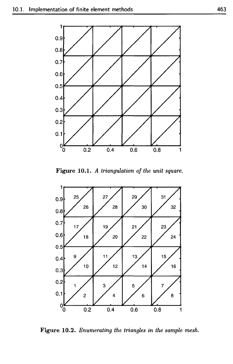
regular triangular mesh,

defined

on the

unit square, consisting

of 32

triangles

and

25

nodes. This mesh

is

shown

in

Figure 10.1.

In

order

to

perform

the

necessary calculations,

we

must know which nodes

are

associated with which triangles.

Of

course, each triangle

has

three nodes;

we

need

to

know

the

indices

of

these three nodes

in the

list

HI,

112,..

-,

HM-

We

define

the

mapping

e

by the

property

that

the

nodes

of

triangle

Tj

are

n

e

(

i;1

),

n

e

(j

;2

),

n

e

(i,3)

•

(So

e is a

function

of two

variables;

the first

must take

an

integral value

from

1 to

L,

and the

second

one of the

integers

1,2,3.)

In

our

sample mesh, there

are 32

triangles

(L =

32),

and

they

are

enumerated

as in

Figure 10.2.

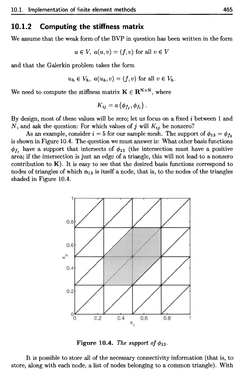
The M = 25

nodes

are

enumerated

as

shown

in

Figure 10.3, which

explicitly shows

the

indices

of the

nodes belonging

to

each triangle.

For

example,

expressing

the

fact

that

the

vertices

of

triangle

10 are

nodes

6, 7, and 12.

Each

of the

standard

basis

functions

for the

space

of

continuous piecewise

linear

functions

corresponds

to one

node

in the

triangulation.

The

basis

functions

75

If

the

domain

fi has

curved boundaries, then,

in the

context

of

piecewise

linear

finite

elements,

the

boundary must

be

approximated

by a

polygonal

curve

made

up of

edges

of

triangles. This

introduces

an

additional error into

the

approximation. When

using

higher-order

finite

elements,

for

example,

piecewise

quadratic

or

piecewise

cubic

functions,

then

it is

straightforward

to

approximate

the

boundary

by a

piecewise

polynomial curve

of the

same degree

as is

used

for the finite

element

functions.

This technique

is

called

the

isoparametric

method,

and it

leads

to a

significant

reduction

in

the

error.

We

will

ignore

all

such questions

here

by

restricting ourselves

to

polygonal domains.

462

Chapter 10.

More

about finite element methods

• Efficient computation of

the

various integrals

that

define

the

entries in the

stiffness matrix

and

load vector.

• Algorithms for assembling

the

stiffness matrix

and

the load vector.

We

will now discuss these issues.

10.1.1

Describing

a triangulation

Before

we

can describe

data

structures and algorithms,

we

must develop notation

for

the

computational mesh. First of all,

we

will assume

that

the

domain n on

which

the

BVP

is

posed

is

a bounded polygonal domain in R2,

so

that

it can be

triangulated.

75

Let

Th

= {Ti : i =

1,2,

...

,

L}

be the collection of triangles in the mesh under consideration,

and

let

Nh

=

{llj

: j =

I,2,

...

,M}

be

the

set of nodes of

the

triangles in

Th.

(Standard notation in finite element

methods labels each mesh with

h,

the

length of the longest side of any triangle in

the

mesh. Similarly,

the

space of piecewise linear functions relative

to

that

mesh

is

denoted

Vh,

and

an arbitrary element of

Vh

as

Vh.

We

will now adopt this standard

notation.)

To

make this discussion as concrete as possible,

we

will use as an example a

regular triangular mesh, defined on

the

unit square, consisting of 32 triangles and

25

nodes. This mesh

is

shown in Figure IO.1.

In

order to perform

the

necessary calculations,

we

must know which nodes are

associated with which triangles. Of course, each triangle has three nodes;

we

need

to

know

the

indices of these three nodes in

the

list

lll,

ll2,

...

,

llM.

We

define

the

mapping e by the property

that

the

nodes of triangle

Ti

are

lle(i,1),lle(i,2),lle(i,3).

(So e is a function of two variables;

the

first must take an integral value from 1

to

L,

and the second one of the integers

1,2,3.)

In

our sample mesh, there are 32 triangles (L = 32),

and

they are enumerated

as in Figure

10.2. The M =

25

nodes are enumerated as shown in Figure 10.3, which

explicitly shows

the

indices of

the

nodes belonging

to

each triangle. For example,

e(IO,

1)

==

6, e(IO,2)

==

7,

e(1O,3) = 12,

expressing the fact

that

the

vertices of triangle

10

are nodes

6,

7,

and

12.

Each of

the

standard basis functions for

the

space of continuous piecewise

linear functions corresponds to one node in the triangulation. The basis functions

751f

the

domain

n has curved boundaries,

then,

in

the

context

of

piecewise linear finite elements,

the

boundary

must

be

approximated

by a polygonal curve

made

up

of

edges

of

triangles.

This

introduces

an

additional

error

into

the

approximation.

When

using higher-order finite elements, for

example, piecewise

quadratic

or

piecewise cubic functions,

then

it

is straightforward

to

approximate

the

boundary

by

a piecewise polynomial curve

of

the

same

degree as is used for

the

finite element

functions.

This

technique is called

the

isopammetric

method,

and

it

leads

to

a significant reduction

in

the

error. We will ignore all such questions here

by

restricting ourselves

to

polygonal domains.

10.1.

Implementation

of

finite element methods

463

Figure

10.1.

A

triangulation

of

the

unit square.

Figure

10.2.

Enumerating

the

triangles

in the

sample

mesh.

10.1.

Implementation

of finite

element

methods

463

Figure

10.1.

A triangulation

of

the unit square.

Figure

10.2.

Enumerating the triangles in the sample mesh.

464

Chapter

10.

More about finite element methods

Figure

10.3. Enumerating

the

nodes

in the

sample mesh.

correspond

to the

degrees

of

freedom

in the finite

element approximation. However,

not

every node

in the

triangulation

need give rise

to a

degree

of

freedom; some

may

be

associated with Dirichlet boundary conditions which determine

the

weight

given

to the

corresponding

basis

function.

For

this reason,

it is not

sufficient

to

identify

the set of all

nodes

in the

triangulation;

we

must also determine

the

free

nodes—those

that

do not

correspond

to a

Dirichlet condition.

We

will

label

the

free

nodes

as

n^,

n/

2

,...,

n/^.

Referring

again

to the

sample mesh

of

Figure

10.1,

if we

assume

that

this mesh

will

be

used

in a

Dirichlet problem, only

the

interior nodes correspond

to

degrees

of

freedom.

Thus

N = 9 and the

free

nodes

can be

enumerated

in the

same order

as the set of all

nodes (left-to-right

and

bottom-to-top).

This yields

We

now

define

the

standard

basis

function

fa by the

conditions

that

fa is a

continuous piecewise linear

function

relative

to the

mesh

7ft,

and

The finite

element

space—the

space

of

continuous piecewise linear functions

(relative

to the

mesh

7ft)

that

satisfy

any

given homogeneous Dirichlet

conditions—

is

then

464

Chapter

10.

More about finite element methods

25

20

15

10

0.1

5

0.2 0.4

Figure

10.3.

Enumerating the nodes in the sample mesh.

correspond

to

the degrees of freedom in the finite element approximation. However,

not every node in the triangulation need give rise

to

a degree of freedom; some

may be associated with Dirichlet boundary conditions which determine the weight

given

to

the

corresponding basis function. For this reason, it

is

not sufficient

to

identify the set of all nodes in

the

triangulation;

we

must also determine the free

nodes-those

that

do not correspond

to

a Dirichlet condition.

We

will label

the

free

nodes as

ll/l,ll/2,

...

,llfN.

Referring again

to

the

sample mesh of Figure 10.1, if

we

assume

that

this mesh

will be used in a Dirichlet problem, only the interior nodes correspond

to

degrees

of freedom. Thus

N = 9 and

the

free nodes can be enumerated in the same order

as the set of all nodes (left-to-right and bottom-to-top). This yields

It

=

7,

h = 8, h =

9,

/4

= 12,

15

= 13,

16

= 14, h = 17,

Is

= 18, fg =

19.

We

now define

the

standard basis function

¢>i

by the conditions

that

¢>i

is a

continuous piecewise linear function relative

to

the mesh

1h,

and

A.

( )

J:

{I,

i =

j,

'l'i

lli

=

Vii

= 0 .

...J..

, Z r J.

The finite element

space-the

space of continuous piecewise linear functions

(relative

to

the

mesh

1h)

that

satisfy any given homogeneous Dirichlet

conditions-

is

then

10.1. Implementation

of

finite

element methods

465

By

design, most

of

these values

will

be

zero;

let us

focus

on a fixed i

between

1 and

AT,

and ask the

question:

For

which

values

of j

will

KIJ

be

nonzero?

As

an

example, consider

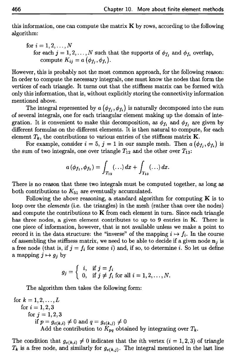
i — 5 for our

sample mesh.

The

support

of

^13

=

0/

5

is

shown

in

Figure 10.4.

The

question

we

must answer

is:

What

other basis

functions

(f>f

j

have

a

support

that

intersects

of

^13

(the intersection must have

a

positive

area;

if the

intersection

is

just

an

edge

of a

triangle, this

will

not

lead

to a

nonzero

contribution

to

K).

It is

easy

to see

that

the

desired basis

functions

correspond

to

nodes

of

triangles

of

which

1113

is

itself

a

node,

that

is, to the

nodes

of the

triangles

shaded

in

Figure 10.4.

Figure

10.4.

The

support

0/^13.

It is

possible

to

store

all of the

necessary connectivity information

(that

is, to

store, along with each node,

a

list

of

nodes belonging

to a

common triangle). With

10.1.2

Computing

the

stiffness

matrix

We

assume

that

the

weak

form

of the

B

VP in

question

has

been written

in the

form

and

that

the

Galerkin

problem takes

the

form

We

need

to

compute

the

stiffness

matrix

K €

R

NxN

,

where

10.1. Implementation

of

finite element methods 465

10.1.2 Computing the stiffness matrix

We

assume

that

the weak form of

the

BVP in question has been written in the form

u E

V,

a(u,v)

=

(f,v)

for all v E V

and

that

the

Galerkin problem takes the form

We

need

to

compute the stiffness matrix K E R

NXN

, where

By design, most of these values will be zero; let us focus on a fixed

i between 1

and

N,

and ask the question: For which values of j will

Kij

be nonzero?

As

an example, consider i = 5 for our sample mesh. The support of

CP13

=

cP

16

is

shown in Figure lOA. The question

we

must answer

is:

What

other basis functions

CPt;

have a support

that

intersects of

CP13

(the intersection must have a positive

area; if the intersection

is

just an edge of a triangle, this will not lead

to

a nonzero

contribution to

K).

It

is

easy

to

see

that

the desired basis functions correspond

to

nodes of triangles of which

n13

is

itself a node,

that

is,

to

the nodes of

the

triangles

shaded in Figure

lOA.

Figure

10.4.

The support

of

CP13.

It

is

possible

to

store all of the necessary connectivity information

(that

is,

to

store, along with each node, a list of nodes belonging

to

a common triangle).

With

466

Chapter

10.

More about

finite

element methods

this information,

one can

compute

the

matrix

K by

rows, according

to the

following

algorithm:

for

i =

1,2,...,N

for

each

j =

l,2,...,N

such

that

the

supports

of

(f)f

j

and

(f>f

t

overlap,

compute

Kij = a

(<j>f.,

0^).

However,

this

is

probably

not the

most common approach,

for the

following

reason:

In

order

to

compute

the

necessary integrals,

one

must

know

the

nodes

that

form

the

vertices

of

each triangle.

It

turns

out

that

the

stiffness

matrix

can be

formed

with

only

this

information,

that

is,

without explicitly storing

the

connectivity information

mentioned above.

The

integral represented

by a

(0^.,

<}>f.)

is

naturally decomposed into

the sum

of

several integrals,

one for

each triangular element making

up the

domain

of

inte-

gration.

It is

convenient

to

make this decomposition,

as

<j>f

4

and

0^.

are

given

by

different

formulas

on the

different

elements.

It is

then natural

to

compute,

for

each

element

Tk, the

contributions

to

various entries

of the

stiffness

matrix

K.

For

example,

consider

%

= 5, j = 1 in our

sample mesh.

Then

a

((f>f^

0/J

is

the sum of two

integrals,

one

over triangle

T

i2

and the

other over

Ti

3

:

There

is no

reason

that

these

two

integrals must

be

computed together,

as

long

as

both contributions

to

K

5

i

are

eventually accumulated.

Following

the

above reasoning,

a

standard

algorithm

for

computing

K is to

loop

over

the

elements (i.e.

the

triangles)

in the

mesh (rather

than

over

the

nodes)

and

compute

the

contributions

to K

from

each element

in

turn. Since each triangle

has

three nodes,

a

given element contributes

to up to 9

entries

in K.

There

is

one

piece

of

information, however,

that

is not

available unless

we

make

a

point

to

record

it in the

data

structure:

the

"inverse"

of the

mapping

i

t-t

fa. In the

course

of

assembling

the

stiffness

matrix,

we

need

to be

able

to

decide

if a

given node

n^

is

a

free

node

(that

is, if j = fa for

some

i)

and,

if so, to

determine

i. So let us

define

a

mapping

j

•->•

gj by

The

algorithm then takes

the

following

form:

for

A?

=

1,2,...,L

for»

=

1,2,3

for

j

=

1,2,3

if

P =

9e(k,i)

^

0 and q =

g

e(kij)

±

0

Add

the

contribution

to

K

pq

obtained

by

integrating

over

Tk.

The

condition

that

g

e

(k,i)

/

0

indicates

that

the

ith

vertex

(i =

1,2,3)

of

triangle

Tk

is a

free

node,

and

similarly

for

<?

e

(fc,j)

• The

integral mentioned

in the

last

line

466

Chapter 10. More

about

finite element methods

this information, one can compute the matrix K by rows, according

to

the following

algorithm:

for

i = 1,2,

...

, N

for each j = 1,2,

...

, N such

that

the supports of

cPlj

and

cPl.

overlap,

compute

Kij

= a

(cPlj,

cPl.)·

However, this

is

probably not the most common approach,

for

the following reason:

In order

to

compute the necessary integrals, one must know the nodes

that

form the

vertices of each triangle.

It

turns out

that

the stiffness matrix can be formed with

only this information,

that

is, without explicitly storing the connectivity information

mentioned above.

The integral represented by

a

(cP/;,

cPf;)

is

naturally decomposed into the sum

of several integrals, one for each triangular element making up the domain of inte-

gration.

It

is

convenient

to

make this decomposition, as

cPf;

and

cPlj

are given by

different formulas on the different elements.

It

is

then natural to compute, for each

element

T

k

,

the contributions

to

various entries of the stiffness matrix K.

For example, consider i =

5,

j = 1 in our sample mesh. Then a

(cPlj

,

cPl;)

is

the sum of two integrals, one over triangle

T12

and the other over

T13:

There

is

no reason

that

these two integrals must be computed together, as long as

both contributions to

K51

are eventually accumulated.

Following the above reasoning, a standard algorithm for computing

K is

to

loop over the elements

(Le.

the triangles) in the mesh (rather

than

over the nodes)

and compute the contributions

to

K from each element in turn. Since each triangle

has three nodes,

a given element contributes

to

up

to

9 entries in

K.

There

is

one piece of information, however,

that

is

not available unless

we

make a point

to

record it in the

data

structure: the "inverse" of the mapping i f-+

Ii.

In the course

of assembling the stiffness matrix,

we

need

to

be able to decide if a given node

nj

is

a free node (that is, if j =

Ii

for some

i)

and, if so,

to

determine

i.

So

let us define

a mapping j

f-+

gj

by

i,

if j =

Ii

0,

if j

:#

Ii for all i = 1,2,

...

, N.

The algorithm then takes the following form:

for

k =

1,

2,

...

, L

for i =

1,2,3

forj=1,2,3

if p =

ge(k,i)

:#

0 and q =

ge(k,j)

:#

0

Add the contribution

to

Kpq

obtained by integrating over Tk.

The condition

that

ge(k,i)

:#

0 indicates

that

the

ith

vertex (i =

1,2,3)

of triangle

n

is

a free node, and similarly for

ge(k,j).

The integral mentioned in the last line

10.1.

Implementation

of

finite

element methods

467

of

this

algorithm

is the

contribution

to

K

pq

= a

(0

e

(fc,j)>0e(M))

fr°

m

the

element

TV

Also,

it

should

be

pointed

out

that,

in the

case

that

K is

symmetric

(as it is in

the

examples considered

in

this

book),

part

of the

work

can be

eliminated:

we

just

compute

the

entries

K

pq

with

q>p,

and

then assign

the

value

of

K

pq

to

K

qp

.

We

have described above

the

information needed

to

carry

out

this algorithm.

It is

easy

to

store this information

in

arrays

for use in a

computer program.

A

simple

data

structure would consist

of

four

arrays:

76

1.

NodeList:

An M x 2

array;

the iih row

consists

of the x and y

coordinates

of

node

n^.

2.

ElementList:

An L x 3

array;

the

kth

row

consists

of

e(fc,l),e(fc,2),e(fc,3).

3.

FreeNodePtrs:

An N x 1

array;

the iih

entry

is

/j.

4.

NodePtrs:

An M x 1

array;

the iih

entry

is

gi.

By

way of

example, Table 10.1 shows these arrays

for the

sample mesh

of

Figure

10.1.

The

information recorded

in

these arrays

will

suffice

for

straightforward

finite

element problems with homogeneous Dirichlet

or

Neumann boundary conditions

(or

even

for

inhomogeneous Dirichlet

problems—see

Exercise

5). For

problems with

inhomogeneous Neumann conditions,

it may

also

be

necessary

to

record whether

a

given

edge belongs

to the

boundary.

The

ElementList

array

can be

augmented

by

columns containing

flags

indicating whether

the

edges

lie on the

boundary. (Or,

of

course,

these

flags can be

stored

in

independent arrays,

if

desired.)

This

extension

is

left

to the

reader.

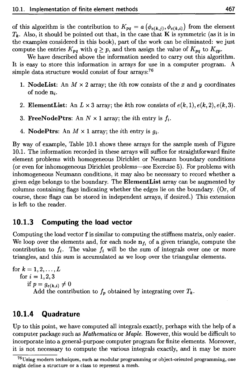
10.1.3

Computing

the

load

vector

Computing

the

load vector

f is

similar

to

computing

the

stiffness

matrix, only easier.

We

loop over

the

elements and,

for

each node

n/

{

of a

given triangle, compute

the

contribution

to

fi.

The

value

fi

will

be the sum of

integrals

over

one or

more

triangles,

and

this

sum is

accumulated

as we

loop over

the

triangular elements.

for

k =

1,2,...,L

for

i =

1,2,3

if

P

=

9e(k,i)

/

0

Add

the

contribution

to

f

p

obtained

by

integrating over

T^.

10.1.4

Quadrature

Up

to

this point,

we

have computed

all

integrals exactly, perhaps with

the

help

of a

computer package such

as

Mathematica

or

Maple.

However, this would

be

difficult

to

incorporate into

a

general-purpose computer program

for finite

elements. Moreover,

it is not

necessary

to

compute

the

various integrals exactly,

and it may be

more

76

Using

modern techniques, such

as

modular programming

or

object-oriented programming,

one

might

define

a

structure

or a

class

to

represent

a

mesh.

10.1. Implementation

of

finite element methods

467

of this algorithm is

the

contribution

to

Kpq

= a

(tPe(k,j)

,

tPe(k,i))

from

the

element

T

k

.

Also, it should be pointed out

that,

in the case

that

K

is

symmetric (as it

is

in

the examples considered in this book),

part

of the work can be eliminated:

we

just

compute

the

entries

Kpq

with q 2 p, and then assign the value of

Kpq

to

Kqp.

We

have described above the information needed

to

carry out this algorithm.

It

is

easy

to

store this information in arrays for use in a computer program. A

simple

data

structure would consist of four arrays: 76

1.

NodeList:

An M x 2 array; the

ith

row consists of

the

x

and

y coordinates

of node

ni.

2.

ElementList:

An L x 3 array; the

kth

row consists of

e(k,1),e(k,2),e(k,3).

3.

FreeNodePtrs:

An N x 1 array;

the

ith

entry

is

k

4.

NodePtrs:

An M x 1 array; the

ith

entry is

gi.

By way of example, Table 10.1 shows these arrays for the sample mesh of Figure

10.1. The information recorded in these arrays will suffice for straightforward finite

element problems with homogeneous Dirichlet or Neumann boundary conditions

(or even for inhomogeneous Dirichlet

problems-see

Exercise 5). For problems with

inhomogeneous Neumann conditions, it may also be necessary

to

record whether a

given edge belongs to the boundary. The

ElementList

array can be augmented by

columns containing flags indicating whether

the

edges

lie

on

the

boundary. (Or, of

course, these flags can be stored in independent arrays, if desired.) This extension

is

left to the reader.

10.1.3 Computing the

load

vector

Computing

the

load vector f

is

similar to computing

the

stiffness matrix, only easier.

We

loop over

the

elements and, for each node

nt.

of a given triangle, compute

the

contribution to

Ii.

The value

Ii

will

be the sum of integrals over one or more

triangles,

and

this sum

is

accumulated as

we

loop over the triangular elements.

for

k = 1,2,

...

, L

for i =

1,2,3

if

p =

ge(k,i)

f:-

0

Add the contribution

to

Ip

obtained by integrating over T

k

·

10.1.4 Quadrature

Up

to

this point,

we

have computed all integrals exactly, perhaps with

the

help of a

computer package such as

Mathematica or

Maple.

However, this would be difficult

to

incorporate into a general-purpose computer program for finite elements. Moreover,

it

is not necessary

to

compute

the

various integrals exactly,

and

it may be more

76Using

modern

techniques, such as

modular

programming

or

object-oriented

programming,

one

might

define a

structure

or

a class

to

represent a mesh.

Gockenbach M.S. Partial Differential Equations. Analytical and Numerical Methods

Подождите немного. Документ загружается.