Gockenbach M.S. Partial Differential Equations. Analytical and Numerical Methods
Подождите немного. Документ загружается.

falls
below some predetermined tolerance
e.
(a)
Write
a
program implementing
the CG
algorithm with
the
above stop-
ping criterion.
(b)
Use
your program
to
solve
the
finite
element equation
Ku
= f
arising
from
the BVP
(10.10)
for
meshes
of
various sizes.
For a fixed
value
of
e,
how
does
the
number
of
iterations required depend
on the
number
of
unknowns
(free
nodes)?
9.
Explain
how the CG
algorithm must
be
modified
if the
initial estimate
x(°)
is
not the
zero vector. (Hint: Think
of
using
the CG
algorithm
to
compute
y
=
x
—
x(°).
What
linear
system
does
y
satisfy?)
10.3
An
outline
of the
convergence theory
for
finite
element methods
We
will
now
present
an
overview
of the
convergence theory
for
Galerkin
finite
ele-
ment methods
for
BVPs.
Our
discussion
is
little
more than
an
outline, describing
the
kinds
of
analysis
that
are
required
to
prove
that
the finite
element method
converges
to the
true solution
as the
mesh
is
refined.
We
will
use the
Dirichlet
problem
as our
model problem.
488
Chapter
10.
More about
finite
element methods
(a)
Perform
one
step
of the
steepest
descent
algorithm,
beginning
at
x(°)
=
(4,2).
Compute
the
steepest
descent direction
at
x(°)
and the
minimizer
along
the
line
defined
by the
steepest descent direction. Compare your
results
to
Figure
10.11.
(b)
Now
compute
the
second step
of the
steepest descent algorithm.
Do you
arrive
at the
exact solution
of Ax
=
b?
(c)
Perform
two
steps
of CG,
beginning with
x(°)
= 0. Do you
obtain
the
exact solution?
8.
When applying
an
iterative method,
a
stopping
criterion
is
essential:
One
must decide,
on the
basis
of
some computable quantity, when
the
computed
solution
is
accurate enough
that
one can
stop
the
iteration.
A
common stop-
ping criterion
is to
stop when
the
relative
residual,
488
Chapter
10.
More
about finite element methods
(a) Perform one step of the steepest descent algorithm, beginning
at
x(O)
=
(4,2). Compute
the
steepest descent direction
at
x(O)
and the minimizer
along the line defined by
the
steepest
descent direction. Compare your
results to Figure 10.1I.
(b) Now compute
the
second step of
the
steepest descent algorithm. Do you
arrive
at
the exact solution of
Ax
=
b?
(c) Perform two steps of CG, beginning with
x(O)
=
o.
Do you obtain the
exact solution?
8. When applying
an
iterative method, a stopping criterion
is
essential: One
must decide, on
the
basis of some computable quantity, when the computed
solution
is
accurate enough
that
one can stop the iteration. A common stop-
ping criterion
is
to
stop when
the
relative residual,
iiAx(k) -
bii
Ilbll
falls below some predetermined tolerance
E.
(a) Write a program implementing
the
CG algorithm with the above stop-
ping criterion.
(b) Use your program
to
solve
the
finite element equation
Ku
= f arising
from
the
BVP
(10.10) for meshes of various sizes. For a fixed value of
E, how does
the
number of iterations required depend on
the
number of
unknowns (free nodes)?
9. Explain how the CG algorithm must
be
modified if the initial estimate
x(O)
is
not the zero vector. (Hint: Think of using the CG algorithm
to
compute
y = x -
x(O).
What
linear system does y satisfy?)
10.3 An outline
of
the convergence theory for finite
element methods
We
will now present
an
overview of the convergence theory for Galerkin finite ele-
ment methods for BVPs. Our discussion
is
little more
than
an
outline, describing
the kinds of analysis
that
are required
to
prove
that
the finite element method
converges
to
the
true
solution as the mesh is refined.
We
will use
the
Dirichlet
problem
as our model problem.
-V'.
(k(x)V'u) =
f(x)
in
0,
u = 0 on
ao
(10.15)
84
The
reader
will
recall
that
the
support
of a
function
is the
closure
of the set on
which
the
function
is
nonzero.
10.3.
An
outline
of the
convergence
theory
for
finite
element methods
489
10.3.1
The
Sobolev
space
H*(n)
We
begin
by
addressing
the
question
of the
proper setting
for the
weak
form of the
BVP.
In
Section 8.4,
we
derived
the
weak
form
as
However,
as we
pointed
out in
Section
5.6
(for
the
one-dimensional case),
the
choice
of
Cf^rj)
for the
space
of
test
functions
is not
really
appropriate
for our
purposes,
since
the
finite
element method uses functions
that
are not
smooth enough
to
belong
to
<?£>(£))
•
Moreover,
the
statement
of the
weak
form
does
not
require
that
the
test
functions
be so
smooth.
We
can
define
the
appropriate space
of
test
functions
by
posing
the
following
question:
What
properties must
the
test
functions
have
in
order
that
the
variational
equation
be
well-defined?
The
energy inner product
is
essentially
the L
2
inner product
of
(the boundary integral must vanish since
0
and all of its
derivatives
are
zero
on the
boundary).
We can
define
a
derivative
of /
G
L
2
(f2)
by
this equation:
If
there
is a
function
g €
L
2
(17)
such
that
An
issue
that
immediately arises
is the
definition
of the
partial
derivatives
of
u.
Need
du/dxi,
du/dx^
exist
at
every point
of
£)?
If so,
then
the use of
piecewise
linear functions
is
still ruled out.
The
classical
definition
of
partial
derivatives
(as
presented
in
calculus books
and
courses),
in
terms
of
limits
of
difference
quotients,
is
purely local. There
is
another
way to
define
derivatives
that
is
more global
in
nature,
and
therefore more
tolerant
of
certain kinds
of
singularities.
We
begin
by
defining
the
space
Co°(tl)
to
be the set of all
infinitely
differentiable
functions
whose
support
84
does
not
intersect
the
boundary
of
fi.
(That
is, the
support
of a
(70°(fJ)
function
is
strictly
in the
interior
of
fi.)
If / is any
smooth
function
defined
on
fK
and
(f>
G
(70°
(fJ),
then,
by
integration
by
parts,
(The
coefficient
of the
PDE,
fc(x), is
also involved. However,
if we
assume
that
k
is
smooth
and
bounded, then,
for the
purposes
of
this discussion,
it may as
well
be
constant
and
therefore
can be
ignored.)
It
suffices,
therefore,
that
the
partial
derivatives
of u and v
belong
to
L
2
(t)},
and it is
natural
to
define
the
space
10.3.
An
outline of the convergence theory
for
finite element methods
489
10.3.1 The Sobolev space
H~(n)
We
begin by addressing the question of
the
proper setting for the weak form of
the
BVP. In Section 8.4,
we
derived
the
weak form as
find
U E
eben)
such
that
a(u,v)
=
(f,v)
for all v E
eben).
(10.16)
However, as
we
pointed out in Section 5.6 (for the one-dimensional case), the choice
of
eb
(n) for the space of test functions
is
not really appropriate for our purposes,
since
the
finite element method uses functions
that
are not smooth enough
to
belong
to
Cb(n).
Moreover, the statement of the weak form does not require
that
the
test
functions be so smooth.
We
can define the appropriate space of test functions by posing the following
question:
What
properties must
the
test functions have in order
that
the variational
equation
a(u,v)
=
(f,v)
be well-defined? The energy inner product
is
essentially
the
L2
inner product of
OU
OV
ou
OV
OXl
OXl
+
OX2 OX2
.
(The coefficient of the PDE, k(x),
is
also involved. However, if
we
assume
that
k
is
smooth and bounded, then, for the purposes of this discussion, it may as
well
be constant and therefore can be ignored.)
It
suffices, therefore,
that
the partial
derivatives of
u and v belong
to
L2(O),
and
it
is
natural
to
define
the
space
(10.17)
An issue
that
immediately arises
is
the definition of the partial derivatives of u.
Need
OU/OX1,
OU/OX2
exist
at
every point of
O?
If
so, then the use of piecewise
linear functions
is
still ruled out.
The classical definition of partial derivatives (as presented in calculus books
and courses), in terms of limits of difference quotients, is purely local. There
is
another way
to
define derivatives
that
is
more global in nature, and therefore more
tolerant of certain kinds of singularities.
We
begin by defining
the
space
C8"(O)
to
be the set of all infinitely differentiable functions whose support
84
does not intersect
the
boundary of
O.
(That
is, the support of a e8"CO) function
is
strictly in the
interior of
0.)
If
f
is
any smooth function defined on 0
and
¢ E C8"(O), then, by
integration by parts,
(10.18)
(the boundary integral must vanish since ¢
and
all of its derivatives are zero on the
boundary).
We
can define a derivative of f E L2(O) by this equation:
If
there
is
a
function g
E L2(O) such
that
r g¢ = - r f
~¢
for all ¢ E
ego(o),
in
in
UXl
84The
reader
will recall
that
the
support
of
a function is
the
closure of
the
set
on
which
the
function is nonzero.
490
Chapter
10.
More about
finite
element methods
then
g is
called
the
(weak)
partial
derivative
of /
with respect
to
x\,
and
denoted
df/dxi.
The
definition
of
df/dx2
in the
weak sense
is
entirely analogous.
We
use the
same notation
for the
weak
partial
derivatives
as we do for the
classical
partial
derivatives;
it can be
proved
that
if the
classical
partial
derivatives
of
/
exist, then
so do the
weak
partial
derivatives,
and the two are the
same.
The
definition
(10.17)
is to be
interpreted
in
terms
of
weak derivatives.
The
space
H
l
(tl)
is an
example
of a
Sobolev
space.
It can be
shown
that
continuous piecewise linear functions belong
to
/f
1
(J7),
while,
for
example, discontinuous piecewise linear functions
do
not. Exercise
2
explores
this
question
in one
dimension;
a
more complete justification
is
beyond
the
scope
of
this book.
The
standard inner product
for
H
l
(tl)
is
and the
induced norm
is
A
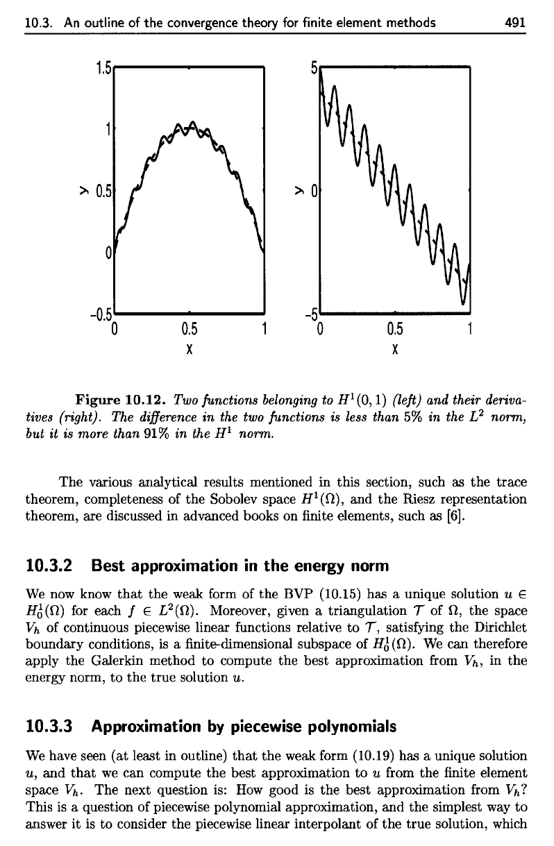
function
g is a
good approximation
to / in the
H
1
sense
if and
only
if g is a
good approximation
to / and
Vg
is a
good approximation
to
V#.
If we
were
to
measure closeness
in the L
2
norm,
on the
other hand,
V#
need
not be
close
to
V/.
For
an
example
of the
distinction
(in one
dimension, which
is
easier
to
visualize),
see
Figure
10.12.
Just
as the
expression
a(u,
v)
makes sense
as
long
as
u
and v
belong
to
H
l
(0),
the
right-hand side
(/, v) of the
variational
equation
is
well-defined
as
long
as /
belongs
to
L
2
(f2).
It is in
this sense
that
the
variational equation
a(u,v)
=
(f,v)
is
called
the
weak
form
of the
BVP:
the
equation
makes
sense
under relatively weak
assumptions
on the
functions involved.
We
now
define
the
subspace
#o(fJ)
of
H
l
(ft)
by
Then,
by the
so-called
trace
theorem,
HQ
(17)
is a
well-defined
and
closed subspace
of
H
1
^).
Moreover,
it can be
shown
that
H
l
(fl)
(and hence
#Q(^))
is
complete
under
the
H
l
norm. (The notion
of
completeness
was
defined
in
Section 9.6.)
Moreover,
the
energy inner product
is
equivalent
to the
H
1
norm
on the
subspace
HQ($I),
which implies
that
HQ(O,)
is
complete under
the
energy norm
as
well.
It
then
follows
from
the
Riesz representation theorem
that
the
weak
form
of the
BVP,
which
we now
pose
as
has
a
unique
solution
for
each
/
e
L
2
(f2).
When
/ is
continuous
and
there
is a
classical solution
u to the
BVP, then
u is
also
the
unique solution
to the
weak
form
of
the
BVP.
490
Chapter 10.
More
about finite element methods
then
9
is
called
the
(weak) partial derivative of 1 with respect
to
Xl,
and denoted
a 1 / aXI. The definition of a 1/
aX2
in the weak sense
is
entirely analogous.
We
use the same notation for
the
weak partial derivatives as
we
do for
the
classical partial derivatives; it can be proved
that
if
the
classical partial derivatives
of
1 exist, then so do
the
weak partial derivatives, and
the
two are the same. The
definition (10.17)
is
to be interpreted in terms of weak derivatives. The space
HI
(0)
is an example of a Sobolev space.
It
can be shown
that
continuous piecewise linear functions belong
to
HI
(0),
while, for example, discontinuous piecewise linear functions do not. Exercise 2
explores this question in one dimension; a more complete justification
is
beyond
the
scope of this book.
The
standard inner product for
HI(O)
is
i
(
a 1
ag
a 1 a
g
)
(f,g)Hl
=
Ig
+
-a -a
+
-a -a
'
n
Xl Xl
X2
X2
and
the
induced norm
is
A function 9
is
a good approximation
to
1 in the
HI
sense if
and
only if 9
is
a
good approximation
to
1 and
\7
9
is
a good approximation
to
\7
g.
If
we
were
to
measure closeness in the
L2
norm, on the other hand,
\7
9 need not be close
to
\71.
For
an
example of
the
distinction (in one dimension, which is easier
to
visualize),
see Figure 10.12.
Just
as
the
expression a(u, v) makes sense as long as u and v belong
to
HI(O),
the
right-hand side (f,
v)
of the variational equation
is
well-defined as long as 1
belongs to
L2(0).
It
is
in this sense
that
the
variational equation a(u,v) =
(f'v)
is
called
the
weak form of
the
BVP:
the
equation makes sense under relatively weak
assumptions on
the
functions involved.
We
now define
the
subspace HJ(O) of
HI(O)
by
HJ(O)={uEHI(O):
u=OonaO}.
Then, by
the
so-called trace theorem, HJ(O)
is
a well-defined and closed subspace
of
HI(O).
Moreover, it can be shown
that
HI(O)
(and hence HJ(O))
is
complete
under the
HI
norm. (The notion of completeness was defined in Section 9.6.)
Moreover,
the
energy inner product
is
equivalent to the
HI
norm on the subspace
HJ(O), which implies
that
HJ(O) is complete under the energy norm as well.
It
then follows from
the
Riesz representation theorem
that
the weak form of the BVP,
which
we
now pose as
find
u E HJ(O) such
that
a(u,v) =
(f,v)
for all v E HJ(O),
(10.19)
has a unique solution for each 1 E
L2(0).
When f is continuous and there is a
classical solution
u
to
the
BVP, then u
is
also
the
unique solution
to
the weak form
of
the
BVP.
10.3.
An
outline
of the
convergence
theory
for
finite element methods
491
Figure
10.12.
Two
functions
belonging
to
H
l
(Q,
1)
(left)
and
their
deriva-
tives
(right).
The
difference
in the two
functions
is
less
than
5% in the L
2
norm,
but
it is
more than
91% in the
H
1
norm.
The
various analytical results mentioned
in
this section, such
as the
trace
theorem, completeness
of the
Sobolev space
H
l
(£t),
and the
Riesz representation
theorem,
are
discussed
in
advanced books
on finite
elements, such
as
[6].
10.3.2
Best approximation
in the
energy norm
We
now
know
that
the
weak
form
of the BVP
(10.15)
has a
unique solution
u €
HQ($})
for
each
/
e
L
2
(f)).
Moreover, given
a
triangulation
T of
fi,
the
space
Vh
of
continuous piecewise linear functions relative
to T,
satisfying
the
Dirichlet
boundary conditions,
is a finite-dimensional
subspace
of
-ffg(fl).
We can
therefore
apply
the
Galerkin method
to
compute
the
best approximation
from
Vh, in the
energy
norm,
to the
true solution
u.
10.3.3
Approximation
by
piecewise polynomials
We
have seen
(at
least
in
outline)
that
the
weak
form
(10.19)
has a
unique solution
u, and
that
we can
compute
the
best approximation
to u
from
the finite
element
space
Vh. The
next question
is: How
good
is the
best approximation
from
V/j,?
This
is a
question
of
piecewise polynomial approximation,
and the
simplest
way to
answer
it is to
consider
the
piecewise linear
interpolant
of the
true solution, which
10.3.
An
outline
of
the
convergence
theory for finite element methods
1.5,....------"""1
-0.5'---------'
o
0.5
X
5-------"""1
),
0
-5'"-------
o
0.5
X
491
Figure
10.12.
Two functions belonging to HI(O,
1)
(left) and their deriva-
tives (right). The difference in the two functions is less than
5%
in the
L2
norm,
but
it
is
more than
91
% in the
HI
norm.
The various analytical results mentioned in this section, such as
the
trace
theorem, completeness of the Sobolev space
HI(O), and
the
Riesz representation
theorem, are discussed in advanced books on finite elements, such as
[6].
10.3.2 Best approximation
in
the
energy
norm
We
now know
that
the weak form of
the
BVP (10.15) has a unique solution u E
HJ(fl)
for each f E
L2(0).
Moreover, given a triangulation T of fl,
the
space
Vh
of continuous piecewise linear functions relative
to
T, satisfying the Dirichlet
boundary conditions,
is
a finite-dimensional subspace of HJ(O).
We
can therefore
apply the Galerkin method
to
compute the best approximation from V
h
,
in
the
energy norm,
to
the
true
solution u.
10.3.3 Approximation
by
piecewise
polynomials
We
have seen
(at
least in outline)
that
the
weak form (10.19) has a unique solution
u, and
that
we
can compute the best approximation
to
u from the finite element
space
Vh.
The next question is:
How
good
is
the best approximation from
Vh?
This
is
a question of piecewise polynomial approximation, and
the
simplest way
to
answer it
is
to
consider the piecewise linear interpolant of
the
true
solution, which
85
There
are
some restrictions
on the
nature
of the
meshes
TH
as h
—>•
0,
basically
that
the
triangles
do not
become
arbitrarily "skinny."
86
A set fi is
called
convex
if,
whenever
the
endpoints
of a
line
segment
lie in
J7,
then
the
entire
line
segment
lies
in fi.
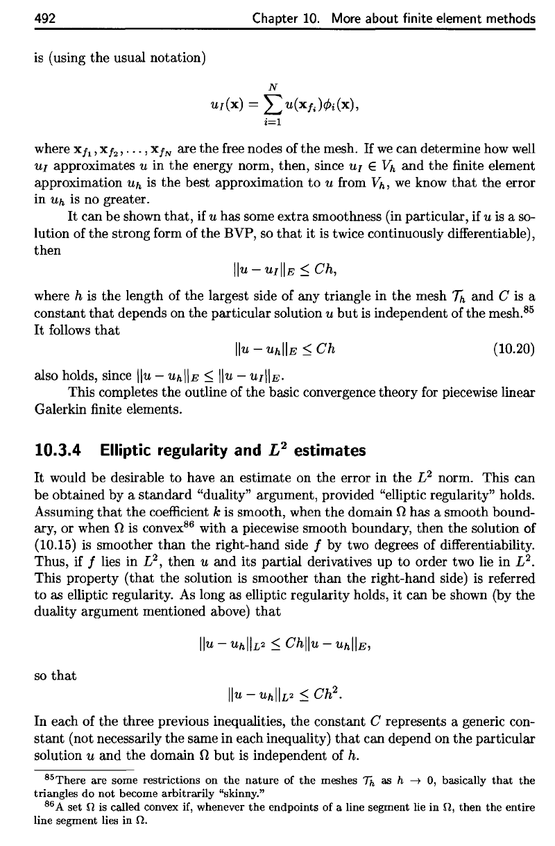
492
Chapter
10.
More about
finite
element methods
is
(using
the
usual notation)
where
x^,
x/
2
,...,
~x.f
N
are the
free
nodes
of the
mesh.
If we can
determine
how
well
HI
approximates
u in the
energy norm, then, since
uj
€
Vh
and the
finite
element
approximation
Uh
is the
best approximation
to u
from
Vh, we
know
that
the
error
in Uh is no
greater.
It can be
shown
that,
if u has
some
extra
smoothness
(in
particular,
if u is a so-
lution
of the
strong
form
of the
BVP,
so
that
it is
twice continuously
differentiable),
then
where
h is the
length
of the
largest side
of any
triangle
in the
mesh
Th
and C is a
constant
that
depends
on the
particular solution
u but is
independent
of the
mesh.
85
It
follows
that
This completes
the
outline
of the
basic convergence theory
for
piecewise linear
Galerkin
finite
elements.
also
holds, since
10.3.4
Elliptic regularity
and
L
2
estimates
It
would
be
desirable
to
have
an
estimate
on the
error
in the
L
2
norm. This
can
be
obtained
by a
standard "duality" argument, provided "elliptic regularity" holds.
Assuming
that
the
coefficient
k is
smooth, when
the
domain
£)
has a
smooth bound-
ary,
or
when
£)
is
convex
86
with
a
piecewise smooth boundary, then
the
solution
of
(10.15)
is
smoother
than
the
right-hand side
/ by two
degrees
of
differentiability.
Thus,
if /
lies
in
L
2
,
then
u and its
partial
derivatives
up to
order
two lie in
L
2
.
This property (that
the
solution
is
smoother
than
the
right-hand side)
is
referred
to as
elliptic regularity.
As
long
as
elliptic regularity holds,
it can be
shown
(by the
duality argument mentioned above)
that
so
that
In
each
of the
three previous inequalities,
the
constant
C
represents
a
generic con-
stant
(not necessarily
the
same
in
each inequality)
that
can
depend
on the
particular
solution
u and the
domain
f)
but is
independent
of h.
492
Chapter
10.
More about finite element methods
is
(using
the
usual notation)
N
UI(X)
= L
U(XfJ¢i(X),
i=l
where
X/I,
X/2,'
..
,
XfN
are the free nodes of
the
mesh.
If
we
can determine how
well
UI
approximates U in
the
energy norm, then, since
UI
E
Vh
and
the
finite element
approximation
Uh
is
the best approximation
to
U from
Vh,
we
know
that
the
error
in
Uh
is
no greater.
It
can be shown
that,
if U has some
extra
smoothness (in particular, if U
is
a so-
lution of
the
strong form of
the
BVP, so
that
it
is
twice continuously differentiable),
then
where h
is
the length of the largest side of any triangle in
the
mesh
1h
and C
is
a
constant
that
depends on the particular solution U
but
is
independent of
the
mesh.
85
It
follows
that
(10.20)
also holds, since
\\u
-
Uh\\E
~
\\u
-
UI\\E'
This completes
the
outline of the basic convergence theory for piecewise linear
Galerkin finite elements.
10.3.4 Elliptic regularity
and
L2 estimates
It
would be desirable
to
have an estimate on the error in the L2 norm. This can
be obtained by a standard "duality" argument, provided "elliptic regularity" holds.
Assuming
that
the
coefficient k
is
smooth, when
the
domain 0 has a smooth bound-
ary, or when
0
is
convex
86
with a piecewise smooth boundary, then the solution of
(10.15) is smoother
than
the
right-hand side f by two degrees of differentiability.
Thus, if
f lies in L2, then U
and
its partial derivatives up
to
order two lie in L2.
This property
(that
the solution
is
smoother
than
the right-hand side)
is
referred
to as elliptic regularity.
As
long as elliptic regularity holds,
it
can be shown (by the
duality argument mentioned above)
that
so
that
In each of
the
three previous inequalities, the constant C represents a generic con-
stant
(not necessarily
the
same in each inequality)
that
can depend on
the
particular
solution
U and
the
domain 0
but
is
independent of
h.
85There
are
some restrictions on
the
nature
of
the
meshes
Th
as h -+ 0, basically
that
the
triangles
do
not
become
arbitrarily
"skinny."
86
A
set
0 is called convex if, whenever
the
endpoints
of
a line segment lie
in
0,
then
the
entire
line segment lies in O.

10.3.
An
outline
of the
convergence
theory
for
finite element
methods
493
Exercises
1.
Suppose
0 €
Co*(ti)
and / :
fi
->•
R is
smooth. Prove
that
for
i =
1,2.
What would
the
boundary integral
be in
this integration
by
parts
formula
if it
were
not
assumed
that
0 is
zero
on
dfi?
2.
The
purpose
of
this exercise
is to
illustrate
why
continuous piecewise linear
functions
belong
to
/^(O,!),
but
discontinuous piecewise linear functions
do
not.
(a)
Define
/ :
[0,1]
-»
R by
Then
/ is
differentiate
(in the
classical sense) everywhere except
at
x
=
1/2,
and
Show
that
/
belongs
to
H
1
(0,1)
and
that
its
weak derivative
is as
defined
above
by
verifying
that
for
every
0
6
C™(Q,
1).
(Hint:
Start
with
the
integral
on the
right,
rewrite
it as the sum of two
integrals,
and
apply integration
by
parts
to
each.)
(b)
Define
g
:
[0,1]
->•
R by
Then
g,
just like
/, is
differentiate
(in the
classical sense) except
at
x
=
1/2,
and
However,
g
£
^
1
(0,1).
Show
that
it is not the
case
that
for
every
0e
C^°(0,l).
10.3.
An
outline
of
the
convergence theory for finite element methods
493
Exercises
1. Suppose
¢>
E
CoCO)
and I : n -+ R
is
smooth. Prove
that
for i = 1,2.
What
would the boundary integral be in this integration by parts
formula if it were not assumed
that
¢>
is
zero on
aO?
2. The purpose of this exercise
is
to
illustrate why continuous piecewise linear
functions belong to
HI
(0,1),
but
discontinuous piecewise linear functions do
not.
(a) Define
I : [0,1] -+ R by
I(x)
= {
x,
I-x,
°
::;
x
::;
~,
~<x::;1.
Then I is differentiable (in
the
classical sense) everywhere except
at
x =
1/2,
and
dl
(x) =
{I,
~
< x <
~,
dx
-1,
2'
< x < 1.
Show
that
I belongs
to
HI
(0,1) and
that
its weak derivative
is
as defined
above by verifying
that
{I
dl
(I
d¢>
io
dx
(x)¢>(x)
dx
= -
io
I(x)
dx
(x)
dx
for every
¢>
E Co(O, 1). (Hint:
Start
with
the
integral on
the
right,
rewrite it
aB
the sum of two integrals, and apply integration by parts
to
each.)
(b) Define
9 : [0,1] -+ R by
g(x)
= {
x,
2-x,
°
::;
x
::;
~,
~<x::;1.
Then g,
just
like
I,
is
differentiable (in
the
claBsical sense) except
at
x =
1/2,
and
dg
(x) = { 1,
dx
-1,
0<
x <
~,
~<x<1.
However, 9 ¢ HI(O, 1). Show
that
it is not
the
CaBe
that
{I
dg
(I
d¢>
io
dx
(x)¢>(x)
dx
= -
io
g(x)
dx
(x)
dx
for every
¢>
E
CoCO,
1).
10.4
Finite
element methods
for
eigenvalue problems
In
Section 9.7,
we
described
how
eigenvalues
and
eigenfunctions exist
for
noncon-
stant
coefficients
problems
on
(more
or
less) arbitrary domains,
but we
gave
no
techniques
for finding
them.
We
will
now
show
how finite
element methods
can
be
used
to
estimate
eigenpairs.
This
will
be a fitting
topic
to end
this book,
as it
ties together
our two
main themes: (generalized) Fourier series methods
and finite
element methods.
We
will
consider
the
following
model problem:
494
Chapter
10.
More about finite element methods
3. Let
f]
be the
unit square
and
define
/, g €
H
l
(ty
by
Compute
the
relative
difference
in / and g in the L
2
and
H
1
norms.
4.
The
exact solution
of the BVP
is
u(x)
=
x
3
(l
—
x).
Consider
the
regular mesh with three elements,
the
subintervals
[0,1/3],
[1/3,2/3],
and
[2/3,1].
(a)
Compute
the
piecewise linear
finite
element approximation
to
u,
and
call
it
v.
(b)
Compute
the
piecewise linear
interpolant
of w, and
call
it
w.
(c)
Compute
the
error
in v and w (as
approximations
to
u)
in the
energy
norm. Which
is
smaller?
We
follow
the
usual procedure
to
derive
the
weak
form:
multiply
by a
test
function,
and
integrate
by
parts:
494
Chapter 10.
More
about finite element methods
3. Let 0 be the unit square
and
define
I,g
E HI(O) by
I(x)
= 1 +
Xl
+
X2,
g(x) =
I(x)
+ sin (m1fXI) sin (n1fX2).
Compute
the
relative difference in 1 and 9 in the
L2
and HI norms.
4.
The exact solution of
the
BVP
cPu
2
--
= 12x - 6x 0 < X < 1
dx
2
' ,
u(O)
= 0,
u(l)
= 0
is
u(x)
= x
3
(1
- x). Consider the regular mesh with three elements, the
subintervals
[0,1/3]'
[1/3,2/3],
and [2/3,1].
(a) Compute the piecewise linear finite element approximation
to
u, and call
it
v.
(b) Compute the piecewise linear interpolant of u, and call
it
w.
(c)
Compute the error in v and w (as approximations
to
u)
in the energy
norm. Which
is
smaller?
10.4 Finite element methods for eigenvalue
problems
In Section 9.7,
we
described how eigenvalues and eigenfunctions exist for noncon-
stant coefficients problems on (more or less) arbitrary domains,
but
we
gave no
techniques for finding them.
We
will now show how finite element methods can
be used
to
estimate eigenpairs. This will be a fitting topic
to
end this book, as it
ties together our two main themes: (generalized) Fourier series methods and finite
element methods.
We
will consider the following model problem:
-V'.
(k(x)V'u) =
Au
in
0,
u = 0 on
ao.
(10.21)
We
follow
the
usual procedure
to
derive
the
weak form: multiply by a
test
function,
and integrate by parts:
-V'.
(k(x)V'u) =
AU,
x E 0
~
-V'.
(k(x)V'u) v =
AUV,
x E
0,
v E H6(O)
~
-
In
V'
. (k(x)V'u) v = A
In
uv, v E H6(O)
~
In
k(x)V'u·
V'v
= A
In
uv, v E HJ(O).
10.4.
Finite
element methods
for
eigenvalue problems
495
In
the
last
step,
the
boundary term vanishes because
of the
boundary conditions
satisfied
by the
test
function
v. The
weak
form
of the
eigenvalue problem
is
therefore
We
now
apply
Galerkin's
method with piecewise linear
finite
elements.
We
write
Vh
for the
space
of
continuous piecewise linear
functions,
satisfying Dirichlet
conditions, relative
to a
given mesh
7ft.
As
usual,
{0i,02,
• • •
,(f>
n
}
will
represent
the
standard
basis
for
Vh-
Galerkin's method
now
reduces
to
or
to
Substituting
the
formula
for
Uh,
we
obtain
where
K 6
R
nxn
and M
e
R
nxn
are the
stiffness
and
mass matrices, respectively,
encountered
before.
If we find A and
u
satisfying
Ku
=
AMu,
then
A and the
corresponding piecewise linear
function
Uh
will
approximate
an
eigenpair
of the
differential
operator.
We
do not
have
the
space here
to
discuss
the
accuracy
of
eigenvalues
and
eigenfunctions
approximated
by
this method;
the
analysis depends
on the
theory
that
was
only sketched
in the
previous section. Only
the
smaller eigenvalues com-
puted
by the
above method
will
be
reliable estimates
of the
true eigenvalues.
To
keep
our
discussion
on an
elementary level,
we
will
restrict
our
attention
to the
computation
of the
smallest eigenvalue.
(The
reader
will
recall
that
this smallest
eigenvalue
can be
quite important,
for
example,
in
mechanical vibrations.
It
defines
the
fundamental
frequency
of a
system modeled
by the
wave equation.)
Given
two
matrices
K
e
R
nxn
and M
e
R
nxn
,
the
problem
is
called
a
generalized
eigenvalue
problem.
It can be
converted
to an
ordinary eigen-
value problem
in a
couple
of
ways.
For
example, when
M is
invertible, then multi-
plying
both sides
of the
equation
by
M""
1
yields
10.4. Finite element methods for eigenvalue problems
495
In
the
last step, the boundary
term
vanishes because of the boundary conditions
satisfied by
the
test function v.
The
weak form of the eigenvalue problem
is
therefore
U E
HJ(O),
a(u,v) =
A(U,V)
for all v E
HJ(O).
(10.22)
We
now apply Galerkin's method with piecewise linear finite elements.
We
write V
h
for
the
space of continuous piecewise linear functions, satisfying Dirichlet
conditions, relative to a given mesh
'Th.
As
usual,
{</h,¢2,
...
,¢n} will represent
the
standard
basis for
Vh.
Galerkin's method now reduces
to
or
to
n
Uh
=
2:
Clj¢j,
a(uh' ¢i) =
A(Uh'
¢i), i = 1,2,
...
, n.
j=l
Substituting
the
formula for
Uh,
we
obtain
n n
=>
2:
a(¢j,
¢i)CXj
= A
2:(¢j,
¢i)CXj,
i = 1,2,
...
, n
j=l
j=l
=>
Ku=
AMu,
where K E
Rnxn
and
ME
Rnxn
are the stiffness and mass matrices, respectively,
encountered before.
If
we
find A and u satisfying
Ku
= AMu, then A and the
corresponding piecewise linear function
Uh
will approximate an eigenpair of
the
differential operator.
We
do not have the space here
to
discuss the accuracy of eigenvalues and
eigenfunctions approximated by this method; the analysis depends on
the
theory
that
was only sketched in
the
previous section. Only
the
smaller eigenvalues com-
puted by the above method will be reliable estimates of the
true
eigenvalues. To
keep our discussion on
an
elementary level,
we
will restrict our attention
to
the
computation of the smallest eigenvalue. (The reader will recall
that
this smallest
eigenvalue can be quite important, for example, in mechanical vibrations.
It
defines
the
fundamental frequency of a system modeled by
the
wave equation.)
Given two matrices K
E R
nxn
and M E R
nxn
, the problem
u
ERn,
U
1:-
0,
A E
C,
Ku
=
AMu
is
called a generalized eigenvalue problem.
It
can be converted to
an
ordinary eigen-
value problem in a couple of ways. For example, when M
is
invertible, then multi-
plying
both
sides of the equation by
M-
1
yields
496
Chapter
10.
More about
finite
element methods
which
is the
ordinary eigenvalue problem
for the
matrix
M
1
K.
However, this
transformation
has
several drawbacks,
not the
least
of
which
is
that
M
-1
K
will
usually
not be
symmetric even
if
both
K and M are
symmetric. (The reader should
recall
that
symmetric matrices have many special properties with respect
to the
eigenvalue problem: real eigenvalues, orthogonal eigenvectors, etc.)
The
preferred method
for
converting
Ku
=
AMu
into
an
ordinary eigenvalue
problem uses
the
Cholesky factorization
.
Every
SPD
matrix
can be
written
as
the
product
of a
nonsingular
lower triangular matrix times
its
transpose.
The
mass matrix, being
a
Gram matrix,
is SPD
(see Exercise 10.2.6),
so
there exists
a
nonsingular lower triangular matrix
L
such
that
M =
LL
T
.
We can
then rewrite
the
problem
as
follows:
This
is an
ordinary eigenvalue problem
for A, and A is
symmetric because
K is.
This
shows
that
the
generalized eigenvalue problem
Ku = AMu has
real eigenval-
ues.
The
eigenvectors corresponding
to
distinct eigenvalues
are
orthogonal when
expressed
in the
transformed variable
x, but not
necessarily
in the
original variable
u.
However, given distinct eigenvalues
A and
//
and
corresponding eigenvectors
u
and v, the
piecewise linear
function
Uh
and
Vh
with nodal values given
by u and v
are
orthogonal
in the
L
2
norm (see Exercise
1).
There
is a
drawback
to
using
the
above method
for
converting
the
generalized
eigenvalue problem
to an
ordinary one: There
is no
reason
why A
should
be
sparse,
even
though
K and M are
sparse.
For
this reason,
the
most
efficient
algorithms
for
the
generalized eigenvalue problem
treat
the
problem directly instead
of
using
the
above transformation. However,
the
transformation
is
useful
if one has
access only
to
software
for the
ordinary eigenvalue problem.
Example
10.4.
We
will
estimate
the
smallest eigenvalue
and the
corresponding
eigenfunction
of
the
negative Laplacian
(subject
to
Dirichlet conditions)
on the
unit
square
fi. The
reader
will
recall
that
the
exact
eigenpair
is
We
establish
a
regular
mesh
on
£),
with
2n
2
triangles,
(n+1)
2
nodes,
and
(n—I)
2
free
nodes.
We
compute
the
stiffness
matrix
K and the
mass matrix
M, and
solve
the
generalized
eigenvalue problem using
the
function
eig
from
MATLAB.
The
results,
for
various values
ofn,
are
shown
in
Table
10.3.
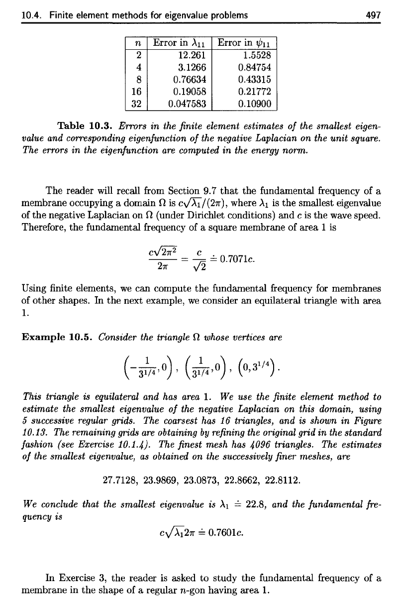
The
reader
should
notice that
the
eigenvalue
estimate
is
converging
faster than
the
eigenfunction
estimate.
This
is
typical.
As the
results suggest,
the
error
in the
eigenvalue
is
O(h
2
),
while
the
error
in the
eigenfunction
is
O(h)
(measured
in the
energy
norm).
496
Chapter 10. More
about
finite element methods
which is the ordinary eigenvalue problem for the matrix
M-1K.
However, this
transformation has several drawbacks, not the least of which is
that
M-
1
K will
usually not be symmetric even if
both
K and M are symmetric. (The reader should
recall
that
symmetric matrices have many special properties with respect
to
the
eigenvalue problem: real eigenvalues, orthogonal eigenvectors, etc.)
The preferred method for converting
Ku
=
.AMu
into an ordinary eigenvalue
problem uses
the
Cholesky factorization. Every SPD matrix can be written as
the
product of a nonsingular lower triangular matrix times its transpose. The
mass matrix, being a Gram matrix,
is
SPD (see Exercise 10.2.6),
so
there exists a
nonsingular lower triangular matrix
L such
that
M = LLT.
We
can then rewrite
the
problem as follows:
Ku=.AMu
:::}
Ku
=
.ALLT
U
:::}
L
-lKu
=
.ALT
u
:::}
L
-lKL
-T
(LT
u)
=
.A
(LT u)
:::}
Ax
=
.Ax,
A = L
-lKL
-T,
x = LT
u.
This
is
an
ordinary eigenvalue problem for
A,
and A
is
symmetric because K is.
This shows
that
the generalized eigenvalue problem
Ku
=
.AMu
has real eigenval-
ues. The eigenvectors corresponding
to
distinct eigenvalues are orthogonal when
expressed in the transformed variable
x,
but
not necessarily in
the
original variable
u.
However, given distinct eigenvalues
.A
and
J.1.
and corresponding eigenvectors u
and v, the piecewise linear function
Uh
and
Vh
with nodal values given by u and v
are orthogonal in the
L2
norm (see Exercise 1).
There
is
a drawback to using
the
above method for converting the generalized
eigenvalue problem
to
an ordinary one: There
is
no reason why A should be sparse,
even though K and M are sparse. For this reason, the most efficient algorithms for
the
generalized eigenvalue problem
treat
the problem directly instead of using the
above transformation. However,
the
transformation
is
useful if one has access only
to
software for the ordinary eigenvalue problem.
Example
10.4.
We
will estimate the smallest eigenvalue and the corresponding
eigenfunction
of
the negative Laplacian (subject to Dirichlet conditions) on the
unit
square
n.
The reader will recall
that
the exact eigenpair is
We
establish a regular
mesh
on
n,
with
2n
2
triangles, (n+1)2 nodes,
and
(n-1)2
free
nodes. We compute the stiffness
matrix
K and the mass
matrix
M,
and solve the
genemlized eigenvalue problem using the
function
eig
from
MATLAB.
The results,
for various values
of
n,
are shown
in
Table 10.B. The reader should notice
that
the
eigenvalue estimate is converging faster
than
the eigenfunction estimate. This is
typical.
As
the results suggest, the error
in
the eigenvalue is
O(h
2
),
while the error
in
the eigenfunction is
O(h)
(measured
in
the energy
norm).
497
n
2
4
8
16
32
Error
in AH
12.261
3.1266
0.76634
0.19058
0.047583
Error
in
t/>n
1.5528
0.84754
0.43315
0.21772
0.10900
Table
10.3. Errors
in the finite
element estimates
of
the
smallest
eigen-
value
and
corresponding
eigenfunction
of
the
negative
Laplacian
on the
unit square.
The
errors
in the
eigenfunction
are
computed
in the
energy
norm.
The
reader
will
recall
from
Section
9.7
that
the
fundamental
frequency
of a
membrane occupying
a
domain
17 is
ci/A7/(27r),
where
AI
is the
smallest
eigenvalue
of
the
negative Laplacian
on 17
(under Dirichlet conditions)
and c is the
wave speed.
Therefore,
the
fundamental
frequency
of a
square membrane
of
area
1 is
In
Exercise
3, the
reader
is
asked
to
study
the
fundamental frequency
of a
membrane
in the
shape
of a
regular
n-gon
having
area
1.
10.4.
Finite
element
methods
for
eigenvalue problems
Using
finite
elements,
we can
compute
the
fundamental frequency
for
membranes
of
other
shapes.
In the
next example,
we
consider
an
equilateral triangle with
area
1.
Example
10.5. Consider
the
triangle
17
whose
vertices
are
This
triangle
is
equilateral
and has
area
1. We use the finite
element method
to
estimate
the
smallest eigenvalue
of the
negative
Laplacian
on
this domain, using
5
successive
regular
grids.
The
coarsest
has 16
triangles,
and is
shown
in
Figure
10.13.
The
remaining
grids
are
obtaining
by
refining
the
original
grid
in the
standard
fashion
(see Exercise 10.1.4).
The finest
mesh
has
4096 triangles.
The
estimates
of
the
smallest
eigenvalue,
as
obtained
on the
successively
finer
meshes,
are
27.7128,
23.9869, 23.0873, 22.8662, 22.8112.
We
conclude
that
the
smallest eigenvalue
is
AI
=
22.8,
and the
fundamental fre-
quency
is
10.4. Finite element methods for eigenvalue problems
497
n
Error in Au Error in
'¢u
2
12.261
1.5528
4
3.1266 0.84754
8
0.76634
0.43315
16
0.19058 0.21772
32 0.047583 0.10900
Table
10.3.
Errors in the finite element estimates
of
the smallest eigen-
value and corresponding eigenfunction
of
the negative Laplacian on the
unit
square.
The errors in the eigenfunction
are
computed in the energy norm.
The reader will recall from Section 9.7
that
the
fundamental frequency of a
membrane occupying a domain
n
is
c";>::;/(27r), where
Al
is
the smallest eigenvalue
of
the
negative Laplacian on n (under Dirichlet conditions) and c
is
the wave speed.
Therefore, the fundamental frequency of a square membrane of area 1
is
cv'27r
2
=
.~
==
0.7071c.
27r
v 2
Using finite elements,
we
can compute
the
fundamental frequency for membranes
of other shapes. In
the
next example,
we
consider an equilateral triangle with area
1.
Example
10.5.
Consider the triangle n whose vertices
are
This triangle is equilateral and has
area
1.
We
use the finite element method to
estimate the smallest eigenvalue
of
the negative Laplacian on this domain, using
5 successive regular grids. The coarsest has
16 triangles, and is shown in Figure
10.13. The remaining grids
are
obtaining
by
refining the original grid in the standard
fashion (see Exercise 10.1.4). The finest mesh has 4096 triangles. The estimates
of
the smallest eigenvalue,
as
obtained on the successively finer meshes,
are
27.7128, 23.9869, 23.0873, 22.8662, 22.8112.
We conclude that the smallest eigenvalue
is
Al
==
22.8, and the fundamental fre-
quency is
cA27r
==
0.7601c.
In Exercise
3,
the reader
is
asked
to
study the fundamental frequency of a
membrane in
the
shape of a regular n-gon having area
1.