Greene W.H. Econometric Analysis

Подождите немного. Документ загружается.

CHAPTER 7

✦

Nonlinear, Semiparametric, Nonparametric Regression

199

for by the interaction term, Female × Education. The negative sign on the latter coefﬁcient

is suggestive. But, the total effect would remain ambiguous without the sort of secondary

analysis suggested by the ﬁgure.

Finally, in addition to the quadratic term in age, the model contains an interaction term,

Age × Education. The coefﬁcient is positive and highly signiﬁcant. But, it is far from obvious

how this should be interpreted. In a linear model,

Income = β

+ β

Age + β

Age

+ β

Education + β

Female

+ β

Female × Education + β

Age × Education + ε,

we would ﬁnd that β

= ∂

E[Income|x]/∂ Age ∂Education. That is, the “interaction effect” is

the change in the partial effect of Age associated with a change in Education (or vice versa).

Of course, if β

equals zero, that is, if there is no product term in the model, then there is

no interaction effect—the second derivative equals zero. However, this simple interpretation

usually does not apply in nonlinear models (i.e., in any nonlinear model). Consider our ex-

ponential regression, and suppose that in fact, β

is indeed zero. For convenience, let μ( x)

equal the conditional mean function. Then, the partial effect with respect to Age is

∂μ( x)/∂Age = μ( x) × ( β

+ 2β

Age)

and

∂

μ( x)/∂Age∂Educ = μ( x) × (β

+ 2β

Age)(β

+ β

Female), (7-25)

which is nonzero even if there is no “interaction term” in the model. The interaction effect

in the model that we estimated, which includes the product term, is

∂

E[y|x]/∂Age∂Educ = μ( x) ×[β

+( β

+2β

Age +β

Educ)(β

+β

Female +β

Age)]. (7-26)

At least some of what is being called the interaction effect in this model is attributable entirely

to the fact the model is nonlinear. To isolate the “functional form effect” from the true “inter-

action effect,” we might subtract (7-25) from (7-26) and then reassemble the components:

∂

μ( x)/∂Age∂Educ = μ( x)[(β

+ 2β

Age)(β

+ β

Female)]

+ μ( x)β

[1 + Age( β

+ 2β

) + Educ(β

+ β

Female) + Educ × Age(β

)]. (7-27)

It is clear that the coefﬁcient on the product term bears essentially no relationship to the

quantity of interest (assuming it is the change in the partial effects that is of interest). On the

other hand, the second term is nonzero if and only if β

is nonzero. One might, therefore,

identify the second part with the “interaction effect” in the model. Whether a behavioral

interpretation could be attached to this is questionable, however. Moreover, that would leave

unexplained the functional form effect. The point of this exercise is to suggest that one should

proceed with some caution in interpreting interaction effects in nonlinear models. This sort

of analysis has a focal point in the literature in Ai and Norton (2004). A number of comments

and extensions of the result are to be found, including Greene (2010).

We make one ﬁnal observation about the nonlinear regression. In a loglinear, single-index

function model such as the one analyzed here, one might, “for comparison purposes,” com-

pute simple linear least squares results. The coefﬁcients in the right-hand side of Table 7.3

suggest superﬁcially that nonlinear least squares and least squares are computing completely

different relationships. To uncover the similarity (if there is one), it is useful to consider the

partial effects rather than the coefﬁcients. We found, for example, the partial effect of educa-

tion in the nonlinear model, using the means of the variables, is 0.000925. Although the linear

least squares coefﬁcients are very different, if the partial effect for education is computed for

the linear equation, we ﬁnd −0.00281 − 0.00685(.5) + 0.00055(43.4452) = 0.01766, where

we have used 0.5 for Female. Dividing by 0.35, we obtain 0.0504, which is at least close to

its counterpart in the nonlinear model. As a general result, at least approximately, the linear

least squares coefﬁcients are making this approximation.

200

PART I

✦

The Linear Regression Model

7.2.6 COMPUTING THE NONLINEAR LEAST SQUARES ESTIMATOR

Minimizing the sum of squared residuals for a nonlinear regression is a standard problem

in nonlinear optimization that can be solved by a number of methods. (See Section E.3.)

The method of Gauss–Newton is often used. This algorithm (and most of the sampling

theory results for the asymptotic properties of the estimator) is based on a linear Taylor

series approximation to the nonlinear regression function. The iterative estimator is

computed by transforming the optimization to a series of linear least squares regressions.

The nonlinear regression model is y = h(x, β) +ε. (To save some notation, we have

dropped the observation subscript). The procedure is based on a linear Taylor series

approximation to h(x, β) at a particular value for the parameter vector, β

h(x, β) ≈ h(x, β

) +



k=1

∂h(x, β

)

∂β



− β



. (7-28)

This form of the equation is called the linearized regression model. By collecting terms,

we obtain

h(x, β) ≈



h(x, β

) −



k=1



∂h(x, β

)

∂β







k=1



∂h(x, β

)

∂β



. (7-29)

Let x

equal the kth partial derivative,

∂h(x, β

)/∂β

. For a given value of β

, x

is a

function only of the data, not of the unknown parameters. We now have

h(x, β) ≈



−



k=1





k=1

which may be written

h(x, β) ≈ h

− x

0

+ x

0

β,

which implies that

y ≈ h

− x

0

+ x

0

β + ε.

By placing the known terms on the left-hand side of the equation, we obtain a linear

equation:

= y − h

+ x

0

= x

0

β + ε

. (7-30)

Note that ε

contains both the true disturbance, ε, and the error in the ﬁrst-order Taylor

series approximation to the true regression, shown in (7-29). That is,

= ε +



h(x, β) −

−



k=1



k=1

,

. (7-31)

Because all the errors are accounted for, (7-30) is an equality, not an approximation.

With a value of β

in hand, we could compute y

and x

and then estimate the parameters

of (7-30) by linear least squares. Whether this estimator is consistent or not remains to

be seen.

You should verify that for the linear regression model, these derivatives are the independent variables.

CHAPTER 7

✦

Nonlinear, Semiparametric, Nonparametric Regression

201

Example 7.7 Linearized Regression

For the model in Example 7.3, the regressors in the linearized equation would be

∂h( .)

∂β

= 1,

∂h( .)

∂β

= e

∂h( .)

∂β

= β

With a set of values of the parameters β

= y − h



x, β

, β



+ β

can be linearly regressed on the three pseudoregressors to estimate β

, β

, and β

The linearized regression model shown in (7-30) can be estimated by linear least

squares. Once a parameter vector is obtained, it can play the role of a new β

, and the

computation can be done again. The iteration can continue until the difference between

successive parameter vectors is small enough to assume convergence. One of the main

virtues of this method is that at the last iteration the estimate of (Q

)

−1

will, apart from

the scale factor ˆσ

/n, provide the correct estimate of the asymptotic covariance matrix

for the parameter estimator.

This iterative solution to the minimization problem is

t+1





i=1

0



−1





i=1



− h

+ x

0





= b





i=1

0



−1





i=1



− h





(7-32)

= b

+ (X

0

)

−1

0

= b

+ 

where all terms on the right-hand side are evaluated at b

and e

is the vector of nonlin-

ear least squares residuals. This algorithm has some intuitive appeal as well. For each

iteration, we update the previous parameter estimates by regressing the nonlinear least

squares residuals on the derivatives of the regression functions. The process will have

converged (i.e., the update will be 0) when X

0

is close enough to 0. This derivative

has a direct counterpart in the normal equations for the linear model, X



e = 0.

As usual, when using a digital computer, we will not achieve exact convergence with

0

exactly equal to zero. A useful, scale-free counterpart to the convergence criterion

discussed in Section E.3.6 is δ = e

0

)

−1

0

. [See (7-22).] We note, ﬁnally,

that iteration of the linearized regression, although a very effective algorithm for many

problems, does not always work. As does Newton’s method, this algorithm sometimes

“jumps off” to a wildly errant second iterate, after which it may be impossible to compute

the residuals for the next iteration. The choice of starting values for the iterations can

be crucial. There is art as well as science in the computation of nonlinear least squares

estimates. [See McCullough and Vinod (1999).] In the absence of information about

starting values, a workable strategy is to try the Gauss–Newton iteration ﬁrst. If it

202

PART I

✦

The Linear Regression Model

fails, go back to the initial starting values and try one of the more general algorithms,

such as BFGS, treating minimization of the sum of squares as an otherwise ordinary

optimization problem.

Example 7.8 Nonlinear Least Squares

Example 7.4 considered analysis of a nonlinear consumption function,

C = α + βY

+ ε.

The linearized regression model is

C − ( α

+ β

γ 0

) + (α

1 + β

γ 0

+ γ

γ 0

ln Y) = α + β( Y

γ 0

) + γ (β

γ 0

ln Y) + ε

Combining terms, we ﬁnd that the nonlinear least squares procedure reduces to iterated

regression of

= C + γ

ln Y



∂h( .)

∂α

∂h( .)

∂β

∂h( .)

∂γ





⎡

⎣

ln Y

⎤

⎦

Finding the starting values for a nonlinear procedure can be difﬁcult. Simply trying a

convenient set of values can be unproductive. Unfortunately, there are no good rules for

starting values, except that they should be as close to the ﬁnal values as possible (not

particularly helpful). When it is possible, an initial consistent estimator of β will be a good

starting value. In many cases, however, the only consistent estimator available is the one

we are trying to compute by least squares. For better or worse, trial and error is the most

frequently used procedure. For the present model, a natural set of values can be obtained

because a simple linear model is a special case. Thus, we can start α and β at the linear least

squares values that would result in the special case of γ = 1 and use 1 for the starting value

for γ . The iterations are begun at the least squares estimates for α and β and 1 for γ .

The solution is reached in eight iterations, after which any further iteration is merely “ﬁne

tuning” the hidden digits (i.e., those that the analyst would not be reporting to their reader;

“gradient” is the scale-free convergence measure, δ, noted earlier). Note that the coefﬁcient

vector takes a very errant step after the ﬁrst iteration—the sum of squares becomes huge—

but the iterations settle down after that and converge routinely.

Begin NLSQ iterations. Linearized regression.

Iteration = 1; Sum of squares = 1536321.88; Gradient = 996103.930

Iteration = 2; Sum of squares = 0.184780956E+12; Gradient = 0.184780452E+12 (×10

)

Iteration = 3; Sum of squares = 20406917.6; Gradient = 19902415.7

Iteration = 4; Sum of squares = 581703.598; Gradient = 77299.6342

Iteration = 5; Sum of squares = 504403.969; Gradient = 0.752189847

Iteration = 6; Sum of squares = 504403.216; Gradient = 0.526642396E-04

Iteration = 7; Sum of squares = 504403.216; Gradient = 0.511324981E-07

Iteration = 8; Sum of squares = 504403.216; Gradient = 0.606793426E-10

7.3 MEDIAN AND QUANTILE REGRESSION

We maintain the essential assumptions of the linear regression model,

y = x



β + ε

where E[ε|x] = 0 and E[y|x] = x



β.Ifε|x is normally distributed, so that the distribution

of ε|x is also symmetric, then the median, Med[ε|x], is also zero and Med[y|x] = x



β.

CHAPTER 7

✦

Nonlinear, Semiparametric, Nonparametric Regression

203

Under these assumptions, least squares remains a natural choice for estimation of β. But,

as we explored in Example 4.5, least absolute deviations (LAD) is a possible alternative

that might even be preferable in a small sample. Suppose, however, that we depart from

the second assumption directly. That is, the statement of the model is

Med[y|x] = x



β.

This result suggests a motivation for LAD in its own right, rather than as a robust (to

outliers) alternative to least squares.

The conditional median of y

might be an inter-

esting function. More generally, other quantiles of the distribution of y

might also be

of interest. For example, we might be interested in examining the various quantiles of

the distribution of income or spending. Quantile regression (rather than least squares)

is used for this purpose. The (linear) quantile regression model can be deﬁned as

Q[y|x, q] = x



such that Prob [y ≤ x



|x] = q, 0 < q < 1. (7-33)

The median regression would be deﬁned for q =

. Other focal points are the lower and

upper quartiles, q =

and q =

, respectively. We will develop the median regression

in detail in Section 7.3.1, once again largely as an alternative estimator in the linear

regression setting.

The quantile regression model is a richer speciﬁcation than the linear model that we

have studied thus far, because the coefﬁcients in (7-33) are indexed by q. The model is

nonparametric—it requires a much less detailed speciﬁcation of the distribution of y|x.

In the simplest linear model with ﬁxed coefﬁcient vector, β, the quantiles of y|x would

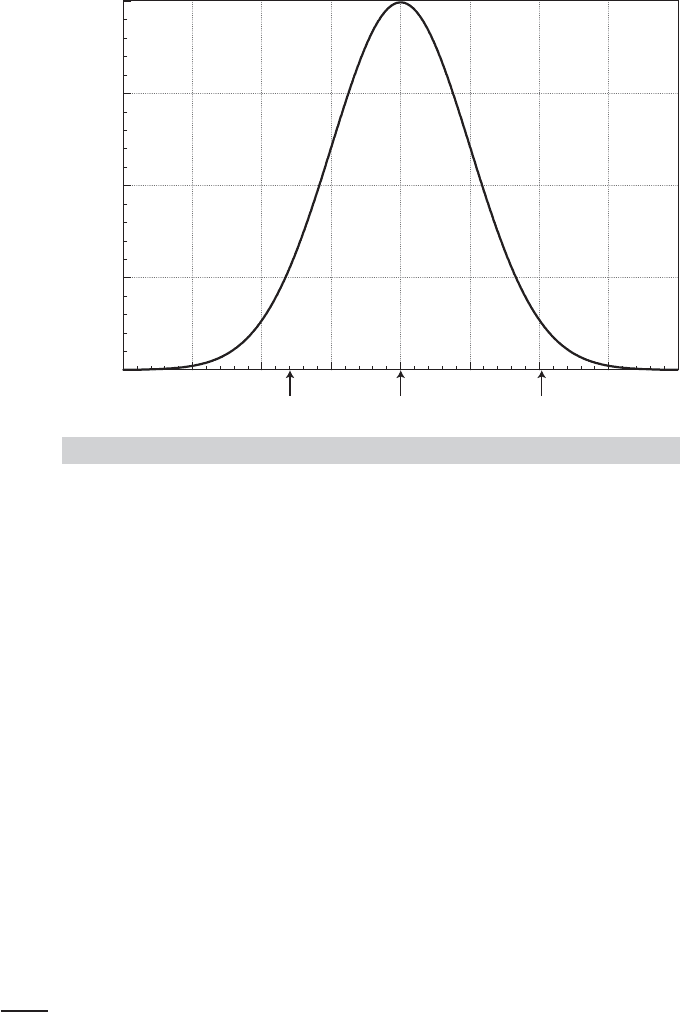
be deﬁned by variation of the constant term. The implication of the model is shown in

Figure 7.4. For a ﬁxed β and conditioned on x, the value of α

+βx such that Prob(y <

+βx) is shown for q = 0.15, 0.5, and 0.9 in Figure 7.4. There is a value of α

for each

quantile. In Section 7.3.2, we will examine the more general speciﬁcation of the quantile

regression model in which the entire coefﬁcient vector plays the role of α

in Figure 7.4.

7.3.1 LEAST ABSOLUTE DEVIATIONS ESTIMATION

Least squares can be severely distorted by outlying observations. Recent applications

in microeconomics and ﬁnancial economics involving thick-tailed disturbance distribu-

tions, for example, are particularly likely to be affected by precisely these sorts of obser-

vations. (Of course, in those applications in ﬁnance involving hundreds of thousands of

observations, which are becoming commonplace, this discussion is moot.) These appli-

cations have led to the proposal of “robust” estimators that are unaffected by outlying

observations.

In this section, we will examine one of these, the least absolute devia-

tions, or LAD estimator.

That least squares gives such large weight to large deviations from the regression

causes the results to be particularly sensitive to small numbers of atypical data points

when the sample size is small or moderate. The least absolute deviations (LAD) esti-

mator has been suggested as an alternative that remedies (at least to some degree) the

In Example 4.5, we considered the possibility that in small samples with possibly thick-tailed disturbance

distributions, the LAD estimator might have a smaller variance than least squares.

For some applications, see Taylor (1974), Amemiya (1985, pp. 70–80), Andrews (1974), Koenker and Bassett

(1978), and a survey written at a very accessible level by Birkes and Dodge (1993). A somewhat more rigorous

treatment is given by Hardle (1990).

204

PART I

✦

The Linear Regression Model

Q (y|x)



0.15

 x 

0.50

 x 

0.90

 x

0.10

0.20

0.30

0.40

Quantiles for a Symmetric Distribution

0.00

Density of y

FIGURE 7.4

Quantile Regression Model.

problem. The LAD estimator is the solution to the optimization problem,

Min



i=1

− x



The LAD estimator’s history predates least squares (which itself was proposed over

200 years ago). It has seen little use in econometrics, primarily for the same reason that

Gauss’s method (LS) supplanted LAD at its origination; LS is vastly easier to compute.

Moreover, in a more modern vein, its statistical properties are more ﬁrmly established

than LAD’s and samples are usually large enough that the small sample advantage of

LAD is not needed.

The LAD estimator is a special case of the quantile regression:

Prob[y

≤ x



] = q.

The LAD estimator estimates the median regression. That is, it is the solution to the

quantile regression when q =0.5. Koenker and Bassett (1978, 1982), Huber (1967), and

Rogers (1993) have analyzed this regression.

Their results suggest an estimator for

the asymptotic covariance matrix of the quantile regression estimator,

Est. Asy. Var[b

] = (X



−1



DX(X



−1

Powell (1984) has extended the LAD estimator to produce a robust estimator for the case in which data on

the dependent variable are censored, that is, when negative values of y

are recorded as zero. See Melenberg

and van Soest (1996) for an application. For some related results on other semiparametric approaches to

regression, see Butler et al. (1990) and McDonald and White (1993).

CHAPTER 7

✦

Nonlinear, Semiparametric, Nonparametric Regression

205

where D is a diagonal matrix containing weights



f (0)



if y

− x



β is positive and



1 − q

f (0)



otherwise,

and f (0) is the true density of the disturbances evaluated at 0.

[It remains to obtain an

estimate of f (0).] There is a useful symmetry in this result. Suppose that the true density

were normal with variance σ

. Then the preceding would reduce to σ

(π/2)(X



−1

which is the result we used in Example 4.5. For more general cases, some other empirical

estimate of f (0) is going to be required. Nonparametric methods of density estimation

are available [see Section 12.4 and, e.g., Johnston and DiNardo (1997, pp. 370–375)].

But for the small sample situations in which techniques such as this are most desir-

able (our application below involves 25 observations), nonparametric kernel density

estimation of a single ordinate is optimistic; these are, after all, asymptotic results.

But asymptotically, as suggested by Example 4.5, the results begin overwhelmingly

to favor least squares. For better or worse, a convenient estimator would be a ker-

nel density estimator as described in Section 12.4.1. Looking ahead, the computation

would be

f (0) =



i=1





where h is the bandwidth (to be discussed shortly), K[.] is a weighting, or kernel function

and e

, i = 1,...,n is the set of residuals. There are no hard and fast rules for choosing

h; one popular choice is that used by Stata (2006), h = .9s/n

1/5

. The kernel function

is likewise discretionary, though it rarely matters much which one chooses; the logit

kernel (see Table 12.2) is a common choice.

The bootstrap method of inferring statistical properties is well suited for this ap-

plication. Since the efﬁcacy of the bootstrap has been established for this purpose,

the search for a formula for standard errors of the LAD estimator is not really neces-

sary. The bootstrap estimator for the asymptotic covariance matrix can be computed as

follows:

Est. Var[b

LAD

] =



r=1

LAD

(r) − b

LAD

)(b

LAD

(r) − b

LAD

)



where b

LAD

is the LAD estimator and b

LAD

(r) is the rth LAD estimate of β based on

a sample of n observations, drawn with replacement, from the original data set.

Example 7.9 LAD Estimation of a Cobb–Douglas Production Function

Zellner and Revankar (1970) proposed a generalization of the Cobb–Douglas production func-

tion that allows economies of scale to vary with output. Their statewide data on Y =value

added (output), K =capital, L =labor, and N =the number of establishments in the trans-

portation industry are given in Appendix Table F7.2. For this application, estimates of the

Koenker suggests that for independent and identically distributed observations, one should replace d

with the constant a =q(1 −q)/[ f (F

−1

(q))]

=[.50/ f (0)]

for the median (LAD) estimator. This reduces the

expression to the true asymptotic covariance matrix, a(X



−1

. The one given is a sample estimator which

will behave the same in large samples. (Personal communication to the author.)

206

PART I

✦

The Linear Regression Model

2

1

3

Residual

Observation Number

8 12 16 20 24 28

MAME

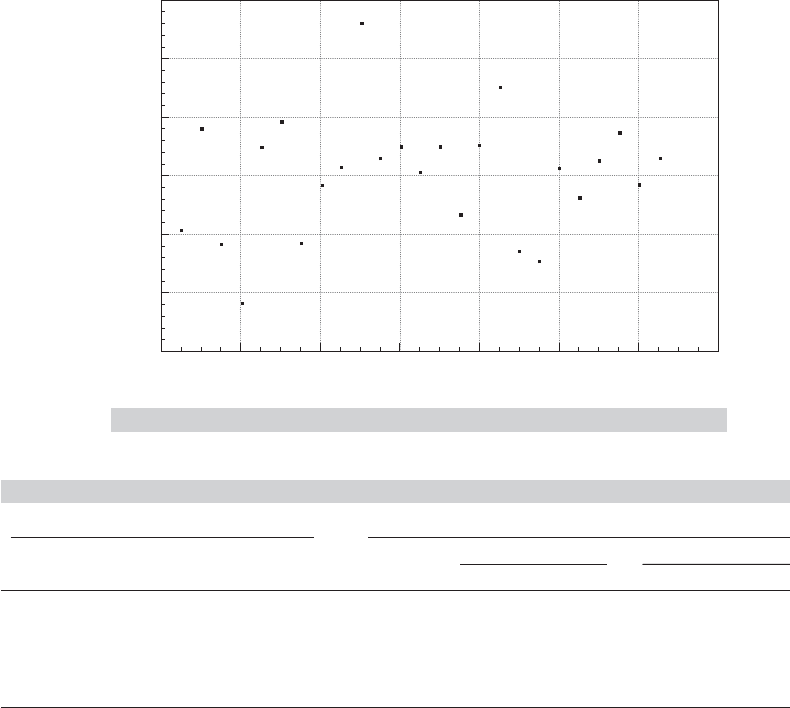
FIGURE 7.5

Standardized Residuals for Production Function.

TABLE 7.4

LS and LAD Estimates of a Production Function

Least Squares LAD

Bootstrap Kernel Density

Coefﬁcient Estimate

Standard

Error t Ratio Estimate Std. Error t Ratio Std. Error t Ratio

Constant 2.293 0.107 21.396 2.275 0.202 11.246 0.183 12.374

0.279 0.081 3.458 0.261 0.124 2.099 0.138 1.881

0.927 0.098 9.431 0.927 0.121 7.637 0.169 5.498

e

0.7814 0.7984

|e| 3.3652 3.2541

Cobb–Douglas production function,

ln(Y

) = β

+ β

ln( K

) + β

ln( L

) + ε

are obtained by least squares and LAD. The standardized least squares residuals shown in

Figure 7.5 suggest that two observations (Florida and Kentucky) are outliers by the usual

construction. The least squares coefﬁcient vectors with and without these two observations

are (2.293, 0.279, 0.927) and (2.205, 0.261, 0.879), respectively, which bears out the sug-

gestion that these two points do exert considerable inﬂuence. Table 7.4 presents the LAD

estimates of the same parameters, with standard errors based on 500 bootstrap replica-

tions. The LAD estimates with and without these two observations are identical, so only

the former are presented. Using the simple approximation of multiplying the corresponding

OLS standard error by (π/2)

1/2

=1.2533 produces a surprisingly close estimate of the boot-

strap estimated standard errors for the two slope parameters (0.102, 0.123) compared with

the bootstrap estimates of (0.124, 0.121). The second set of estimated standard errors are

based on Koenker’s suggested estimator, .25/

(0) = 0.25/1.5467

= 0.104502. The band-

width and kernel function are those suggested earlier. The results are surprisingly consistent

given the small sample size.

CHAPTER 7

✦

Nonlinear, Semiparametric, Nonparametric Regression

207

7.3.2 QUANTILE REGRESSION MODELS

The quantile regression model is

Q[y|x, q] = x



such that Prob[y ≤ x



|x] = q, 0 < q < 1.

This is essentially a nonparametric speciﬁcation. No assumption is made about the

distribution of y|x or about its conditional variance. The fact that q can vary continuously

(strictly) between zero and one means that there are an inﬁnite number of possible

“parameter vectors.” It seems reasonable to view the coefﬁcients, which we might write

β(q) less as ﬁxed “parameters,” as we do in the linear regression model, than loosely

as features of the distribution of y|x. For example, it is not likely to be meaningful to

view β(.49) to be discretely different from β(.50) or to compute precisely a particular

difference such as β(.5)−β(.3). On the other hand, the qualitative difference, or possibly

the lack of a difference, between β(.3) and β(.5) as displayed in our following example,

may well be an interesting characteristic of the sample.

The estimator,b

of β

for a speciﬁc quantile is computed by minimizing the function

(β

|y, X) =



i:y

≥x



q|y

− x





i:y



(1 − q)|y

− x





i=1



− x





where

g(e

i,q

|q) =



i,q

if e

i,q

≥ 0

(1 − q)e

i,q

if e

i,q

< 0



, e

i,q

= y

− x



When q = 0.5, the estimator is the least absolute deviations estimator we examined in

Example 4.5 and Section 7.3.1. Solving the minimization problem requires an iterative

estimator. It can be set up as a linear programming problem.

[See Keonker and D’Oray

(1987).]

We cannot use the methods of Chapter 4 to determine the asymptotic covariance

matrix of the estimator. But, the fact that the estimator is obtained by minimizing a sum

does lead to a set of results similar to those we obtained in Section 4.4 for least squares.

[See Buchinsky (1998).] Assuming that the regressors are “well behaved,” the quantile

regression estimator of β

is consistent and asymptotically normally distributed with

asymptotic covariance matrix

Asy.Var .[b

] =

−1

where

H = plim



i=1

(0|x



Quantile regression is supported as a built in procedure in contemporary software such as Statas, SAS,

and NLOGIT.

208

PART I

✦

The Linear Regression Model

and

G = plim

q(1 − q)



i=1



This is the result we had earlier for the LAD estimator, now with quantile q instead of

0.5. As before, computation is complicated by the need to compute the density of ε

zero. This will require either an approximation of uncertain quality or a speciﬁcation of

the particular density, which we have hoped to avoid. The usual approach, as before, is

to use bootstrapping.

Example 7.10 Income Elasticity of Credit Card Expenditure

Greene (1992, 2007) analyzed the default behavior and monthly expenditure behavior of a

large sample (13,444 observations) of credit card users. Among the results of interest in the

study was an estimate of the income elasticity of the monthly expenditure. A conventional

regression approach might be based on

Q[ln Spending|x, q] = β

1,q

+ β

2,q

ln Income + β

3,q

Age + β

4,q

Dependents.

The data in Appendix Table F7.3 contain these and numerous other covariates that might

explain spending; we have chosen these three for this example only. The 13,444 observations

in the data set are based on credit card applications. Of the full sample, 10,499 applications

were approved and the next 12 months of spending and default behavior were observed.

Spending is the average monthly expenditure in the 12 months after the account was initiated.

Average monthly income and number of household dependents are among the demographic

data in the application. Table 7.5 presents least squares estimates of the coefﬁcients of

the conditional mean function as well as full results for several quantiles.

Standard errors

are shown for the least squares and median (1 = 0.5) results. The results for the other

quantiles are essentially the same. The least squares estimate of 1.08344 is slightly and

signiﬁcantly greater than one—the estimated standard error is 0.03212 so the t statistic is

(1.08344 −1) /0.03212 = 2.60. This suggests an aspect of consumption behavior that might

not be surprising. However, the very large amount of variation over the range of quantiles

might not have been expected. We might guess that at the highest levels of spending for

any income level, there is (comparably so) some saturation in the response of spending to

changes in income.

Figure 7.6 displays the estimates of the income elasticity of expenditure for the range

of quantiles from 0.1 to 0.9, with the least squares estimate which would correspond to

the ﬁxed value at all quantiles shown in the center of the ﬁgure. Conﬁdence limits shown

in the ﬁgure are based on the asymptotic normality of the estimator. They are computed

as the estimated income elasticity plus and minus 1.96 times the estimated standard error.

Figure 7.7 shows the implied quantile regressions for q = 0.1, 0.3, 0.5, 0.7, and 0.9. The

relatively large increase from the 0.1 quantile to the 0.3 suggests some skewness in the

The expenditure data are taken from the credit card records while the income and demographic data are

taken from the applications. While it might be tempting to use, for example, Powell’s (1986a,b) censored

quantile regression estimator to accommodate this large cluster of zeros for the dependent variable, this

approach would misspecify the model—the “zeros” represent nonexistent observations, not missing ones. A

more detailed approach—the one used in the 1992 study—would model separately the presence or absence

of the observation on spending and then model spending conditionally on acceptance of the application. We

will revisit this issue in Chapter 19 in the context of the sample selection model. The income data are censored

at 100,000 and 220 of the observations have expenditures that are ﬁlled with $1 or less. We have not “cleaned”

the data set for these aspects. The full 10,499 observations have been used as they are in the original data set.

We would note, if (7-33) is the statement of the model, then it does not follow that that the conditional

mean function is a linear regression. That would be an additional assumption.