Greene W.H. Econometric Analysis

Подождите немного. Документ загружается.

CHAPTER 7

✦

Nonlinear, Semiparametric, Nonparametric Regression

209

TABLE 7.5

Estimated Quantile Regression Models

Estimated Parameters

Quantile Constant ln Income Age Dependents

0.1 −6.73560 1.40306 −0.03081 −0.04297

0.2 −4.31504 1.16919 −0.02460 −0.04630

0.3 −3.62455 1.12240 −0.02133 −0.04788

0.4 −2.98830 1.07109 −0.01859 −0.04731

(Median) 0.5 −2.80376 1.07493 −0.01699 −0.04995

Std.Error (0.24564) (0.03223) (0.00157) (0.01080)

t −11.41 33.35 −10.79 −4.63

Least Squares −3.05581 1.08344 −0.01736 −.04461

Std.Error (0.23970) (0.03212) (0.00135) (0.01092)

t −12.75 33.73 −12.88 −4.08

0.6 −2.05467 1.00302 −0.01478 −0.04609

0.7 −1.63875 0.97101 −0.01190 −0.03803

0.8 −0.94031 0.91377 −0.01126 −0.02245

0.9 −0.05218 0.83936 −0.00891 −0.02009

Quantile

0.74

0.98

1.22

1.46

1.70

0.50

0.20 0.40 0.60 0.80 1.000.00

Elasticity and Confidence Limits

Elast. Upper Lower Least Squares

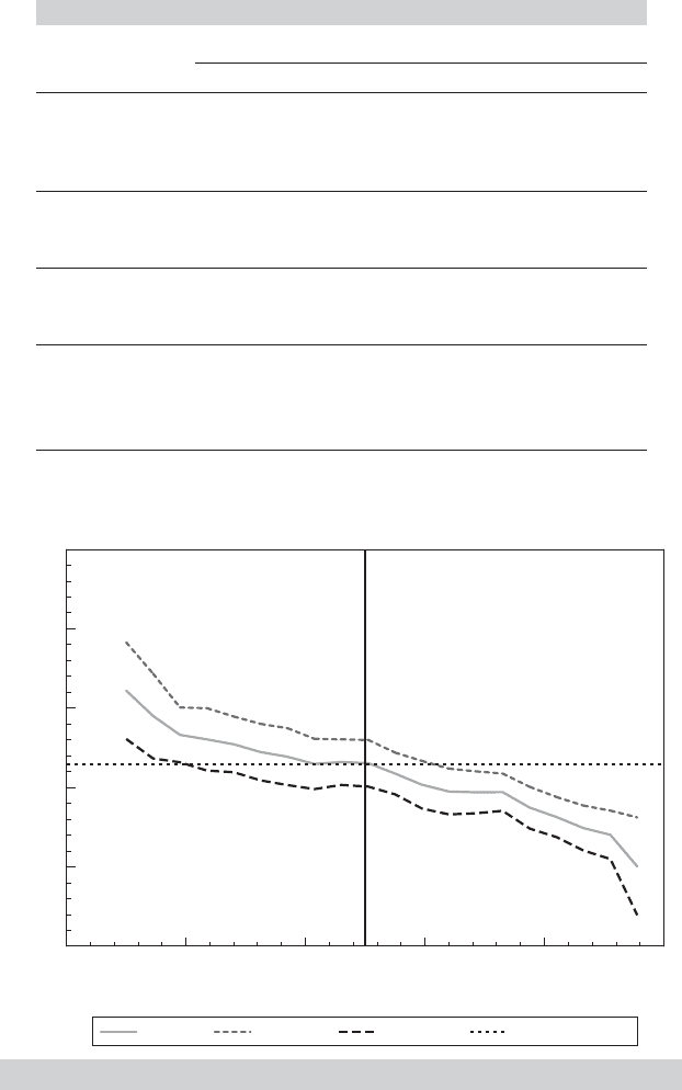
FIGURE 7.6

Estimates of Income Elasticity of Expenditure.

spending distribution. In broad terms, the results do seem to be largely consistent with our

earlier result of the quantiles largely being differentiated by shifts in the constant term, in

spite of the seemingly large change in the coefﬁcient on ln Income in the results.

210

PART I

✦

The Linear Regression Model

1.00

0.50

2.00

3.50

5.00

2.50

4.24 4.68 5.12 5.56 6.003.80

Regression Quantile

Q1 Q3 Q5 Q7 Q9

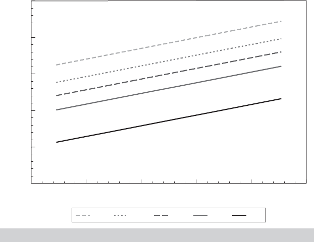
FIGURE 7.7

Quantile Regressions for Ln Spending.

7.4 PARTIALLY LINEAR REGRESSION

The proper functional form in the linear regression is an important speciﬁcation issue.

We examined this in detail in Chapter 6. Some approaches, including the use of dummy

variables, logs, quadratics, and so on, were considered as means of capturing nonlin-

earity. The translog model in particular (Example 2.4) is a well-known approach to

approximating an unknown nonlinear function. Even with these approaches, the re-

searcher might still be interested in relaxing the assumption of functional form in the

model. The partially linear model [analyzed in detail by Yatchew (1998, 2000) and

H¨ardle, Liang, and Gao (2000)] is another approach. Consider a regression model in

which one variable, x, is of particular interest, and the functional form with respect to

x is problematic. Write the model as

= f (x

) + z



β + ε

where the data are assumed to be well behaved and, save for the functional form, the

assumptions of the classical model are met. The function f (x

) remains unspeciﬁed. As

stated, estimation by least squares is not feasible until f (x

) is speciﬁed. Suppose the

data were such that they consisted of pairs of observations (y

, y

), j = 1,...,n/2,

in which x

= x

within every pair. If so, then estimation of β could be based on the

simple transformed model

− y

= (z

− z

)



β + (ε

− ε

), j = 1,...,n/2.

As long as observations are independent, the constructed disturbances, v

still have zero

mean, variance now 2σ

, and remain uncorrelated across pairs, so a classical model

applies and least squares is actually optimal. Indeed, with the estimate of β, say,

CHAPTER 7

✦

Nonlinear, Semiparametric, Nonparametric Regression

211

hand, a noisy estimate of f (x

) could be estimated with y

−z



(the estimate contains

the estimation error as well as ε

The problem, of course, is that the enabling assumption is heroic. Data would not

behave in that fashion unless they were generated experimentally. The logic of the

partially linear regression estimator is based on this observation nonetheless. Suppose

that the observations are sorted so that x

< x

< ···< x

. Suppose, as well, that this

variable is well behaved in the sense that as the sample size increases, this sorted data

vector more tightly and uniformly ﬁlls the space within which x

is assumed to vary.

Then, intuitively, the difference is “almost” right, and becomes better as the sample size

grows. [Yatchew (1997, 1998) goes more deeply into the underlying theory.] A theory

is also developed for a better differencing of groups of two or more observations. The

transformed observation is y

d,i



m=0

i−m

where



m=0

= 0 and



m=0

= 1.

(The data are not separated into nonoverlapping groups for this transformation—we

merely used that device to motivate the technique.) The pair of weights for M = 1is

obviously ±

√

0.5—this is just a scaling of the simple difference, 1, −1. Yatchew [1998,

p. 697)] tabulates “optimal” differencing weights for M =1,...,10. The values for M =2

are (0.8090, −0.500, −0.3090) and for M = 3 are (0.8582, −0.3832, −0.2809, −0.1942).

This estimator is shown to be consistent, asymptotically normally distributed, and have

asymptotic covariance matrix

Asy. Var[

] =



1 +



[Var[z |x]].

The matrix can be estimated using the sums of squares and cross products of the differ-

enced data. The residual variance is likewise computed with

ˆσ



i=M+1

d,i

− z



d,i

)

n − M

Yatchew suggests that the partial residuals, y

d,i

− z



d,i

be smoothed with a kernel

density estimator to provide an improved estimator of f (x

). Manzan and Zeron (2010)

present an application of this model to the U.S. gasoline market.

Example 7.11 Partially Linear Translog Cost Function

Yatchew (1998, 2000) applied this technique to an analysis of scale effects in the costs of

electricity supply. The cost function, following Nerlove (1963) and Christensen and Greene

(1976), was speciﬁed to be a translog model (see Example 2.4 and Section 10.5.2) involving

labor and capital input prices, other characteristics of the utility, and the variable of interest,

the number of customers in the system, C. We will carry out a similar analysis using Chris-

tensen and Greene’s 1970 electricity supply data. The data are given in Appendix Table F4.4.

(See Section 10.5.1 for description of the data.) There are 158 observations in the data set,

but the last 35 are holding companies that are comprised of combinations of the others.

In addition, there are several extremely small New England utilities whose costs are clearly

unrepresentative of the best practice in the industry. We have done the analysis using ﬁrms

6–123 in the data set. Variables in the data set include Q =output, C =total cost, and PK, PL,

and PF =unit cost measures for capital, labor, and fuel, respectively. The parametric model

See Estes and Honor´e (1995) who suggest this approach (with simple differencing of the data).

Yatchew (2000, p. 191) denotes this covariance matrix E [Cov[z |x]].

212

PART I

✦

The Linear Regression Model

speciﬁed is a restricted version of the Christensen and Greene model,

ln c = β

k + β

l + β

q + β

/2) + β

+ ε,

where c = ln[C/( Q × PF )],k = ln(PK/PF),l = ln(PL/PF ), and q = ln Q. The partially linear

model substitutes f (q) for the last three terms. The division by PF ensures that average cost is

homogeneous of degree one in the prices, a theoretical necessity. The estimated equations,

with estimated standard errors, are shown here.

(parametric) c =−7.32 + 0.069k + 0.241 − 0.569q + 0.057q

/2 + ε,

(0.333) (0.065) (0.069) (0.042) (0.006) s = 0.13949

(partially linear) c

= 0.108k

+ 0.163l

+ f (q) + v

(0.076) (0.081) s = 0.16529

7.5 NONPARAMETRIC REGRESSION

The regression function of a variable y on a single variable x is speciﬁed as

y = μ(x) + ε.

No assumptions about distribution, homoscedasticity, serial correlation or, most impor-

tantly, functional form are made at the outset; μ(x) may be quite nonlinear. Because

this is the conditional mean, the only substantive restriction would be that deviations

from the conditional mean function are not a function of (correlated with) x. We have

already considered several possible strategies for allowing the conditional mean to be

nonlinear, including spline functions, polynomials, logs, dummy variables, and so on.

But, each of these is a “global” speciﬁcation. The functional form is still the same for

all values of x. Here, we are interested in methods that do not assume any particular

functional form.

The simplest case to analyze would be one in which several (different) observations

on y

were made with each speciﬁc value of x

. Then, the conditional mean function

could be estimated naturally using the simple group means. The approach has two

shortcomings, however. Simply connecting the points of means, (x

, ¯y |x

) does not

produce a smooth function. The method would still be assuming something speciﬁc

about the function between the points, which we seek to avoid. Second, this sort of data

arrangement is unlikely to arise except in an experimental situation. Given that data

are not likely to be grouped, another possibility is a piecewise regression in which we

deﬁne “neighborhoods” of points around each x of interest and ﬁt a separate linear or

quadratic regression in each neighborhood. This returns us to the problem of continuity

that we noted earlier, but the method of splines, discussed in Section 6.3.1, is actually

designed speciﬁcally for this purpose. Still, unless the number of neighborhoods is quite

large, such a function is still likely to be crude.

Smoothing techniques are designed to allow construction of an estimator of the

conditional mean function without making strong assumptions about the behavior of

the function between the points. They retain the usefulness of the nearest neighbor

concept but use more elaborate schemes to produce smooth, well-behaved functions.

The general class may be deﬁned by a conditional mean estimating function

ˆμ(x

∗

) =



i=1

∗

, x

,...,x



i=1

∗

|x)y

CHAPTER 7

✦

Nonlinear, Semiparametric, Nonparametric Regression

213

where the weights sum to 1. The linear least squares regression line is such an estimator.

The predictor is

ˆμ(x

∗

) = a + bx

∗

where a and b are the least squares constant and slope. For this function, you can show

that

∗

|x) =

∗

− ¯x)



i=1

− ¯x)

The problem with this particular weighting function, which we seek to avoid here, is that

it allows every x

to be in the neighborhood of x

∗

, but it does not reduce the weight of

any x

when it is far from x

∗

. A number of smoothing functions have been suggested that

are designed to produce a better behaved regression function. [See Cleveland (1979)

and Schimek (2000).] We will consider two.

The locally weighted smoothed regression estimator (“loess” or “lowess” depending

on your source) is based on explicitly deﬁning a neighborhood of points that is close to

∗

. This requires the choice of a bandwidth, h.Theneighborhood is the set of points

for which |x

∗

− x

| is small. For example, the set of points that are within the range x*

± h/2 might constitute the neighborhood. The choice of bandwith is crucial, as we will

explore in the following example, and is also a challenge. There is no single best choice.

A common choice is Silverman’s (1986) rule of thumb,

Silver man

.9[min(s, IQR)]

1.349 n

0.2

where s is the sample standard deviation and IQR is the interquartile range (0.75 quan-

tile minus 0.25 quantile). A suitable weight is then required. Cleveland (1979) recom-

mends the tricube weight,

∗

|x, h) =



1 −



− x

∗





Combining terms, then the weight for the loess smoother is

∗

|x, h) = 1(x

in the neighborhood) × T

∗

|x, h).

The bandwidth is essential in the results. A wider neighborhood will produce a

smoother function, but the wider neighborhood will track the data less closely than a

narrower one. A second possibility, similar to the least squares approach, is to allow

the neighborhood to be all points but make the weighting function decline smoothly

with the distance between x* and any x

. A variety of kernel functions are used for this

purpose. Two common choices are the logistic kernel,

K(x

∗

, h) = (v

)[1 − (v

)] where (v

) = exp(v

)/[1 + exp(v

)],v

= (x

− x

∗

)/ h,

214

PART I

✦

The Linear Regression Model

and the Epanechnikov kernel,

K(x

∗

, h) = 0.75(1 − 0.2 v

√

5if|v

|≤5 and 0 otherwise.

This produces the kernel weighted regression estimator,

ˆμ(x

∗

|x, h) =



i=1



− x

∗





i=1



− x

∗



which has become a standard tool in nonparametric analysis.

Example 7.12 A Nonparametric Average Cost Function

In Example 7.11, we ﬁt a partially linear regression for the relationship between average cost

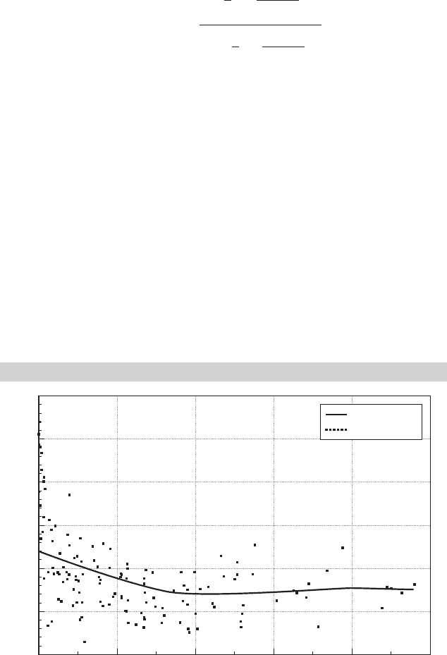
and output for electricity supply. Figures 7.8 and 7.9 show the less ambitious nonparametric

regressions of average cost on output. The overall picture is the same as in the earlier exam-

ple. The kernel function is the logistic density in both cases. The function in Figure 7.8 uses

a bandwidth of 2,000. Because this is a fairly large proportion of the range of variation of

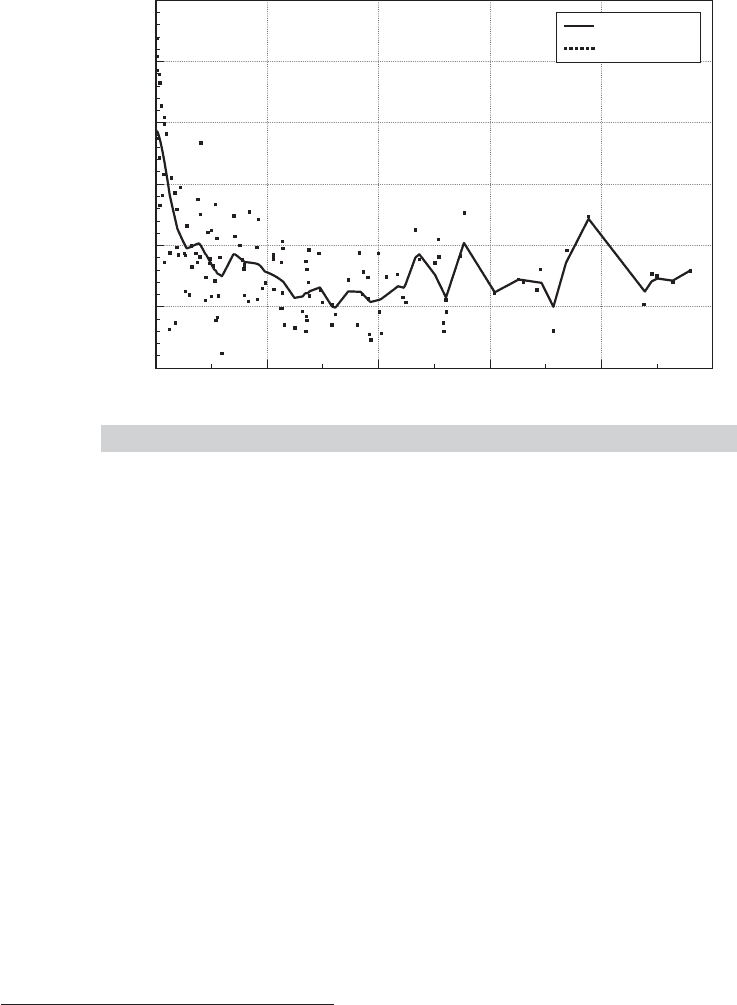
output, the function is quite smooth. The regression in Figure 7.9 uses a bandwidth of only

200. The function tracks the data better, but at an obvious cost. The example demonstrates

what we and others have noted often. The choice of bandwidth in this exercise is crucial.

Data smoothing is essentially data driven. As with most nonparametric techniques,

inference is not part of the analysis—this body of results is largely descriptive. As can

be seen in the example, nonparametric regression can reveal interesting characteristics

of the data set. For the econometrician, however, there are a few drawbacks. There is

no danger of misspecifying the conditional mean function, for example. But, the great

FIGURE 7.8

Nonparametric Cost Function.

0 5,000 10,000 15,000 20,000 25,000

Output

E[AvgCost

AvgCost

CHAPTER 7

✦

Nonlinear, Semiparametric, Nonparametric Regression

215

0 5,000 10,000 15,000 20,000 25,000

Output

E[AvgCost

AvgCost

FIGURE 7.9

Nonparametric Cost Function.

generality of the approach limits the ability to test one’s speciﬁcation or the underlying

theory. [See, for example, Blundell, Browning, and Crawford’s (2003) extensive study

of British expenditure patterns.] Most relationships are more complicated than a simple

conditional mean of one variable. In Example 7.12, some of the variation in average cost

relates to differences in factor prices (particularly fuel) and in load factors. Extensions

of the fully nonparametric regression to more than one variable is feasible, but very

cumbersome. [See H ¨ardle (1990) and Li and Racine (2007).] A promising approach is

the partially linear model considered earlier.

7.6 SUMMARY AND CONCLUSIONS

In this chapter, we extended the regression model to a form that allows nonlinearity

in the parameters in the regression function. The results for interpretation, estimation,

and hypothesis testing are quite similar to those for the linear model. The two crucial

differences between the two models are, ﬁrst, the more involved estimation procedures

needed for the nonlinear model and, second, the ambiguity of the interpretation of the

coefﬁcients in the nonlinear model (because the derivatives of the regression are often

nonconstant, in contrast to those in the linear model).

Key Terms and Concepts

•

Bandwidth

•

Bootstrap

•

Box–Cox transformation

•

Conditional mean function

•

Conditional median

•

Delta method

•

Epanechnikov kernel

•

GMM estimator

•

Identiﬁcation condition

•

Identiﬁcation problem

•

Index function model

•

Indirect utility function

216

PART I

✦

The Linear Regression Model

•

Interaction term

•

Iteration

•

Jacobian

•

Kernel density estimator

•

Kernel functions

•

Least absolute deviations

(LAD)

•

Linear regression model

•

Linearized regression model

•

Lagrange multiplier test

•

Logistic kernel

•

Logit model

•

Loglinear model

•

Median regression

•

Nearest neighbor

•

Neighborhood

•

Nonlinear least squares

•

Nonlinear regression model

•

Nonparametric estimators

•

Nonparametric regression

•

Normalization

•

Orthogonality condition

•

Overidentifying restrictions

•

Partially linear model

•

Pseudoregressors

•

Quantile regression

•

Roy’s identity

•

Semiparametric

•

Semiparametric estimation

•

Silverman’s rule of thumb

•

Smoothing function

•

Starting values

•

Two-step estimation

•

Wald test

Exercises

1. Describe how to obtain nonlinear least squares estimates of the parameters of the

model y = αx

+ ε.

2. Verify the following differential equation, which applies to the Box–Cox transfor-

mation:

(λ)

dλ





(ln x)

−

i−1

(λ)

dλ

i−1



. (7-34)

Show that the limiting sequence for λ = 0is

lim

λ→0

(λ)

dλ

(ln x)

i+1

i + 1

. (7-35)

These results can be used to great advantage in deriving the actual second deriva-

tives of the log-likelihood function for the Box–Cox model.

Applications

1. Using the Box–Cox transformation, we may specify an alternative to the Cobb–

Douglas model as

ln Y = α + β

− 1)

+ β

− 1)

+ ε.

Using Zellner and Revankar’s data in Appendix Table F7.2, estimate α, β

, β

, and

λ by using the scanning method suggested in Example 7.5. (Do not forget to scale

Y, K, and L by the number of establishments.) Use (7-24), (7-15), and (7-16) to

compute the appropriate asymptotic standard errors for your estimates. Compute

the two output elasticities, ∂ ln Y/∂ ln K and ∂ ln Y/∂ ln L, at the sample means of

K and L.(Hint: ∂ ln Y/∂ ln K = K∂ ln Y/∂ K.)

2. For the model in Application 1, test the hypothesis that λ = 0 using a Wald test

and a Lagrange multiplier test. Note that the restricted model is the Cobb–Douglas

loglinear model. The LM test statistic is shown in (7-22). To carry out the test, you

will need to compute the elements of the fourth column of X

, the pseudoregressor

corresponding to λ is ∂ E[y |x]/∂λ |λ = 0. Result (7-35) will be useful.

CHAPTER 7

✦

Nonlinear, Semiparametric, Nonparametric Regression

217

3. The National Institute of Standards and Technology (NIST) has created a web site

that contains a variety of estimation problems, with data sets, designed to test the

accuracy of computer programs. (The URL is http://www.itl.nist.gov/div898/strd/.)

One of the ﬁve suites of test problems is a set of 27 nonlinear least squares prob-

lems, divided into three groups: easy, moderate, and difﬁcult. We have chosen one

of them for this application. You might wish to try the others (perhaps to see if

the software you are using can solve the problems). This is the Misra1c problem

(http://www.itl.nist.gov/div898/strd/nls/data/misra1c.shtml). The nonlinear regres-

sion model is

= h(x, β) + ε

= β



1 −



1 + 2β



+ ε

The data are as follows:

10.07 77.6

14.73 114.9

17.94 141.1

23.93 190.8

29.61 239.9

35.18 289.0

40.02 332.8

44.82 378.4

50.76 434.8

55.05 477.3

61.01 536.8

66.40 593.1

75.47 689.1

81.78 760.0

For each problem posed, NIST also provides the “certiﬁed solution,” (i.e., the right

answer). For the Misralc problem, the solutions are as follows:

Estimate Estimated Standard Error

6.3642725809E +02 4.6638326572E +00

2.0813627256E −04 1.7728423155E −06



e 4.0966836971E −02

= e



e/(n − K) 5.8428615257E −02

Finally, NIST provides two sets of starting values for the iterations, generally one set

that is “far” from the solution and a second that is “close” from the solution. For this

problem, the starting values provided are β

= (500, 0.0001) and β

= (600, 0.0002).

The exercise here is to reproduce the NIST results with your software.[For a detailed

analysis of the NIST nonlinear least squares benchmarks with several well-known

computer programs, see McCullough (1999).]

4. In Example 7.1, the CES function is suggested as a model for production,

lny = lnγ −



δK

−ρ

+ (1 − δ)L

−ρ



+ ε. (7-36)

218

PART I

✦

The Linear Regression Model

Example 6.8 suggested an indirect method of estimating the parameters of this

model. The function is linearized around ρ = 0, which produces an intrinsically

linear approximation to the function,

lny = β

+ β

lnK + β

lnL + β

[1/2(lnK − LnL)

] + ε,

where β

= ln γ,β

= νδ. β

= ν(1 − δ) and β

= ρνδ(1 − δ). The approximation

can be estimated by linear least squares. Estimates of the structural parameters are

found by inverting the preceding four equations. An estimator of the asymptotic

covariance matrix is suggested using the delta method. The parameters of (7-36)

can also be estimated directly using nonlinear least squares and the results given

earlier in this chapter.

Christensen and Greene’s (1976) data on U.S. electricity generation are given

in Appendix Table F4.4. The data ﬁle contains 158 observations. Using the ﬁrst

123, ﬁt the CES production function, using capital and fuel as the two factors of

production rather than capital and labor. Compare the results obtained by the two

approaches, and comment on why the differences (which are substantial) arise.

The following exercises require specialized software. The relevant techniques

are available in several packages that might be in use, such as SAS, Stata, or

LIMDEP. The exercises are suggested as departure points for explorations using a

few of the many estimation techniques listed in this chapter.

5. Using the gasoline market data in Appendix Table F2.2, use the partially linear

regression method in Section 7.4 to ﬁt an equation of the form

ln(G/Pop) = β

ln(Income) + β

lnP

new cars

+ β

lnP

used cars

+ g(lnP

gasoline

) + ε.

6. To continue the analysis in Application 5, consider a nonparametric regression of

G/Pop on the price. Using the nonparametric estimation method in Section 7.5,

ﬁt the nonparametric estimator using a range of bandwidth values to explore the

effect of bandwidth.