Greene W.H. Econometric Analysis
Подождите немного. Документ загружается.

CHAPTER 8
✦
Endogeneity and Instrumental Variables
229
were set in the late 18th through the 19th centuries and handed down to present-day admin-
istrators by historical precedent. In the formative years, the author noted, district boundaries
were set in response to natural travel barriers, such as rivers and streams. It follows, as
she notes, that “the number of districts in a given land area is an increasing function of
the number of natural barriers”; hence, the number of streams in the physical market area
provides the needed instrumental variable. [The controversial topic of the study and the un-
conventional choice of instruments caught the attention of the popular press, for example,
http://gsppi.berkeley.edu/faculty/jrothstein/hoxby/wsj.pdf, and academic observers includ-
ing Rothstein (2004).] This study is an example of a “natural experiment” as described in
Angrist and Pischke (2009).
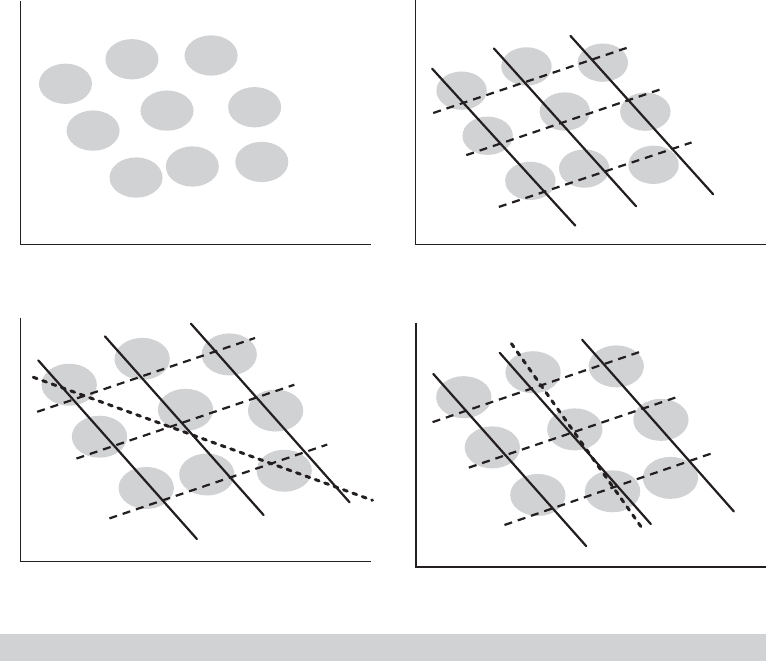
Example 8.4 Instrumental Variable in Regression
The role of an instrumental variable in identifying parameters in regression models was devel-
oped in Working’s (1926) classic application, adapted here for our market equilibrium example
in Example 8.1. Figure 8.1a displays the “observed data” for the market equilibria in a market
in which there are random disturbances (ε
S
, ε
D
) and variation in demanders’ incomes and
input prices faced by suppliers. The market equilibria in Figure 8.1a are scattered about as
the aggregates of all these effects. Figure 8.1b suggests the underlying conditions of sup-
ply and demand that give rise to these equilibria. Different outcomes in the supply equation
(c)
Quantity
Price
S
3
D
1
D
3
D
2
S
2
S
1
(b)
Quantity
Price
S
3
D
1
D
3
D
2
S
2
S
1
(a)
Quantity
Price
(d)
Quantity
Price
S
3
D
1
D
3
D
2
S
2
S
1
FIGURE 8.1
Identifying a Demand Curve with an Instrumental Variable.
230
PART I
✦
The Linear Regression Model
corresponding to different values of the input price and different income values on the demand
side produce nine regimes, punctuated by the random variation induced by the disturbances.
Given the ambiguous mass of points, linear regression of quantity on price (and income) is
likely to produce a result such as that shown by the heavy dotted line in Figure 8.1c. The
slope of this regression barely resembles the slope of the demand equations. Faced with this
prospect, how is it possible to learn about the slope of the demand curve? The experiment
needed, shown in Figure 8.1d, would involve two elements: (1) Hold Income constant, so
we can focus on the demand curve in a particular demand setting. That is the function of
multiple regression—Income is included as a conditioning variable in the equation. (2) Now
that we have focused on a particular set of demand outcomes (e.g., D2), move the supply
curve so that the equilibria now trace out the demand function. That is the function of the
changing InputPrice, which is the instrumental variable that we need for identification of the
demand function(s) for this experiment.
8.3.4 TWO-STAGE LEAST SQUARES
Thus far, we have assumed that the number of instrumental variables in Z is the same as
the number of variables (exogenous plus endogenous) in X. (In the typical application,
the researcher provides the necessary instrumental variable for the single endogenous
variable in their equation.) However, it is possible that the data contain additional
instruments. Recall the market equilibrium application considered in Examples 8.1
and 8.4. Suppose this were an agricultural market in which there are two exogenous
conditions of supply, InputPrice and Rainfall. Then, the equations of the model are
(Demand) Quantity
D
= α
0
+ α
1
Price + α
2
Income + ε
D
,
(Supply) Quantity
S
= β
0
+ β
1
Price + β
2
InputPrice + β
3
Rainfall + ε
S
,
(Equilibrium) Quantity
D
= Quantity
S
.
Given the approach taken in Example 8.4, it would appear that the researcher could
simply choose either of the two exogenous variables (instruments) in the supply equa-
tion for purpose of identifying the demand equation. (We will turn to the now apparent
problem of how to identify the supply equation in Section 8.4.2.) Intuition should sug-
gest that simply choosing a subset of the available instrumental variables would waste
sample information—it seems inevitable that it will be preferable to use the full matrix
Z, even when L > K. The method of two-stage least squares solves the problem of
how to use all the information in the sample when Z contains more variables than are
necessary to construct an instrumental variable estimator.
If Z contains more variables than X, then much of the preceding derivation is
unusable, because Z
X will be L×K with rank K < L and will thus not have an inverse.
The crucial result in all the preceding is plim(Z
ε/n) = 0. That is, every column of Z is
asymptotically uncorrelated with ε. That also means that every linear combination of
the columns of Z is also uncorrelated with ε, which suggests that one approach would
be to choose K linear combinations of the columns of Z. Which to choose? One obvious
possibility, discarded in the preceding paragraph, is simply to choose K variables among
the L in Z. Discarding the information contained in the “extra” L–K columns will turn
out to be inefficient. A better choice is the projection of the columns of X in the column
space of Z:
ˆ
X = Z(Z
Z)
−1
Z
X.
CHAPTER 8
✦
Endogeneity and Instrumental Variables
231
We will return shortly to the virtues of this choice. With this choice of instrumental
variables,
ˆ
X for Z, we have
b
IV
= (
ˆ
X
X)
−1
ˆ
X
y = [X
Z(Z
Z)
−1
Z
X]
−1
X
Z(Z
Z)
−1
Z
y. (8-9)
The estimator of the asymptotic covariance matrix will be ˆσ
2
times the bracketed matrix
in (8-9). The proofs of consistency and asymptotic normality for this estimator are
exactly the same as before, because our proof was generic for any valid set of instruments,
and
ˆ
X qualifies.
There are two reasons for using this estimator—one practical, one theoretical. If
any column of X also appears in Z, then that column of X is reproduced exactly in
ˆ
X. This is easy to show. In the expression for
ˆ
X, if the kth column in X is one of the
columns in Z, say the lth, then the kth column in (Z
Z)
−1
Z
X will be the lth column of
an L × L identity matrix. This result means that the kth column in
ˆ
X = Z(Z
Z)
−1
Z
X
will be the lth column in Z, which is the kth column in X. This result is important and
useful. Consider what is probably the typical application. Suppose that the regression
contains K variables, only one of which, say, the kth, is correlated with the disturbances.
We have one or more instrumental variables in hand, as well as the other K−1 variables
that certainly qualify as instrumental variables in their own right. Then what we would
use is Z = [X
(k)
, z
1
, z
2
,...], where we indicate omission of the kth variable by (k) in
the subscript. Another useful interpretation of
ˆ
X is that each column is the set of fitted
values when the corresponding column of X is regressed on all the columns of Z, which
is obvious from the definition. It also makes clear why each x
k
that appears in Z is
perfectly replicated. Every x
k
provides a perfect predictor for itself, without any help
from the remaining variables in Z. In the example, then, every column of X except the
one that is omitted from X
(k)
is replicated exactly, whereas the one that is omitted is
replaced in
ˆ
X by the predicted values in the regression of this variable on all the z’s.
Of all the different linear combinations of Z that we might choose,
ˆ
X is the most
efficient in the sense that the asymptotic covariance matrix of an IV estimator based on
a linear combination ZF is smaller when F = (Z
Z)
−1
Z
X than with any other F that
uses all L columns of Z; a fortiori, this result eliminates linear combinations obtained
by dropping any columns of Z. This important result was proved in a seminal paper by
Brundy and Jorgenson (1971). [See, also, Wooldridge (2002a, pp. 96–97).]
We close this section with some practical considerations in the use of the instru-
mental variables estimator. By just multiplying out the matrices in the expression, you
can show that
b
IV
= (
ˆ
X
X)
−1
ˆ
X
y
= (X
(I − M
Z
)X)
−1
X
(I − M
Z
)y (8-10)
= (
ˆ
X
ˆ
X)
−1
ˆ
X
y
because I −M
Z
is idempotent. Thus, when (and only when)
ˆ
X is the set of instruments,
the IV estimator is computed by least squares regression of y on
ˆ
X. This conclusion
suggests (only logically; one need not actually do this in two steps), that b
IV
can be
computed in two steps, first by computing
ˆ
X, then by the least squares regression. For
this reason, this is called the two-stage least squares (2SLS) estimator. We will revisit this
form of estimator at great length at several points later, particularly in our discussion of
simultaneous equations models in Section 10.5. One should be careful of this approach,

232
PART I
✦
The Linear Regression Model
however, in the computation of the asymptotic covariance matrix; ˆσ
2
should not be
based on
ˆ
X. The estimator
s
2
IV
=
(y −
ˆ
Xb
IV
)
(y −
ˆ
Xb
IV
)
n
is inconsistent for σ
2
, with or without a correction for degrees of freedom.
An obvious question is where one is likely to find a suitable set of instrumental
variables. The recent literature on “natural experiments” focuses on policy changes such
as the Mariel Boatlift (Example 6.5) or natural outcomes such as occurrences of streams
(Example 8.3) or birthdays [Angrist (1992, 1994)]. In many time-series settings, lagged
values of the variables in the model provide natural candidates. In other cases, the
answer is less than obvious. The asymptotic covariance matrix of the IV estimator can
be rather large if Z is not highly correlated with X; the elements of (Z
X)
−1
grow large.
(See Sections 8.7 and 10.6.6 on “weak” instruments.) Unfortunately, there usually is
not much choice in the selection of instrumental variables. The choice of Z is often ad
hoc.
1
There is a bit of a dilemma in this result. It would seem to suggest that the best
choices of instruments are variables that are highly correlated with X. But the more
highly correlated a variable is with the problematic columns of X, the less defensible
the claim that these same variables are uncorrelated with the disturbances.
Example 8.5 Instrumental Variable Estimation of a Labor Supply
Equation
A leading example of a model in which correlation between a regressor and the disturbance is
likely to arise is in market equilibrium models. Cornwell and Rupert (1988) analyzed the returns
to schooling in a panel data set of 595 observations on heads of households. The sample
data are drawn from years 1976 to 1982 from the “Non-Survey of Economic Opportunity”
from the Panel Study of Income Dynamics. The estimating equation is
ln Wage
it
= β
1
+ β
2
Exp
it
+ β
3
Exp
2
it
+ β
4
Wks
it
+ β
5
Occ
it
+ β
6
Ind
it
+ β
7
South
it
+
β
8
SMSA
it
+ β
9
MS
it
+ β
10
Union
it
+ β
11
Ed
i
+ β
12
Fem
i
+ β
13
Blk
i
+ ε
it
where the variables are
Exp = years of full time work experience,
Wks = weeks worked,
Occ = 1 if blue-collar occupation, 0 if not,
Ind = 1 if the individual works in a manufacturing industry, 0 if not,
South = 1 if the individual resides in the south, 0 if not,
SMSA = 1 if the individual resides in an SMSA, 0 if not,
MS = 1 if the individual is married, 0 if not,
Union = 1 if the individual wage is set by a union contract, 0 if not,
Ed = years of education,
Fem = 1 if the individual is female, 0 if not,
Blk = 1 if the individual is black, 0 if not.
See Appendix Table F8.1 for the data source. The main interest of the study, beyond com-
paring various estimation methods, is β
11
, the return to education. The equation suggested
is a reduced form equation; it contains all the variables in the model but does not spec-
ify the underlying structural relationships. In contrast, the three-equation, model specified
in Section 8.3.4 is a structural equation system. The reduced form for this model would
1
Results on “optimal instruments” appear in White (2001) and Hansen (1982). In the other direction, there
is a contemporary literature on “weak” instruments, such as Staiger and Stock (1997), which we will explore
in Sections 8.7 and 10.6.6.

CHAPTER 8
✦
Endogeneity and Instrumental Variables
233
TABLE 8.1
Estimated Labor Supply Equation
OLS IV with Z
1
IV with Z
2
Variable Estimate Std. Error Estimate Std. Error Estimate Std. Error
Constant 44.7665 1.2153 18.8987 13.0590 30.7044 4.9997
ln Wage 0.7326 0.1972 5.1828 2.2454 3.1518 0.8572
Education −0.1532 0.03206 −0.4600 0.1578 −0.3200 0.06607
Union −1.9960 0.1701 −2.3602 0.2567 −2.1940 0.1860
Female −1.3498 0.2642 0.6957 1.0650 −0.2378 0.4679
consist of separate regressions of Price and Quantity on (1, Income, InputPrice, Rainfall).
We will return to the idea of reduced forms in the setting of simultaneous equations models
in Chapter 10. For the present, the implication for the suggested model is that this market
equilibrium equation represents the outcome of the interplay of supply and demand in a labor
market. Arguably, the supply side of this market might consist of a household labor supply
equation such as
Wks
it
= γ
1
+ γ
2
ln Wage
it
+ γ
3
Ed
i
+ γ
4
Union
it
+ γ
5
Fem
i
+ u
it
.
(One might prefer a different set of right-hand-side variables in this structural equation.)
Structural equations are more difficult to specify than reduced forms. If the number of weeks
worked and the accepted wage offer are determined jointly, then InWage
it
and u
it
in this
equation are correlated. We consider two instrumental variable estimators based on
Z
1
= [1, Ind
it
, Ed
i
, Union
it
, Fem
i
]
and
Z
2
= [1, Ind
it
, Ed
i
, Union
it
, Fem
i
, SMSA
it
].
Table 8.1 presents the three sets of estimates. The least squares estimates are computed
using the standard results in Chapters 3 and 4. One noteworthy result is the very small
coefficient on the log wage variable. The second set of results is the instrumental variable
estimate developed in Section 8.3.2. Note that here, the single instrument is Ind
it
. As might be
expected, the log wage coefficient becomes considerably larger. The other coefficients are,
perhaps, contradictory. One might have different expectations about all three coefficients.
The third set of coefficients are the two-stage least squares estimates based on the larger set
of instrumental variables. In this case, SMSA and Ind are both used as instrumental variables.
8.4 TWO SPECIFICATION TESTS
There are two aspects of the model that we would be interested in verifying if possi-
ble, rather than assuming them at the outset. First, it will emerge in the derivation in
Section 8.4.1 that of the two estimators considered here, least squares and instrumental
variables, the first is unambiguously more efficient. The IV estimator is robust; it is
consistent whether or not plim(X
ε/n) = 0. However, if not needed, that is if γ = 0,
then least squares would be a better estimator by virtue of its smaller variance.
2
For this
reason, and possibly in the interest of a test of the theoretical specification of the model,
2
It is possible, of course, that even if least squares is inconsistent, it might still be more precise. If LS is
only slightly biased but has a much smaller variance than IV, then by the expected squared error criterion,
variance plus squared bias, least squares might still prove the preferred estimator. This turns out to be nearly
impossible to verify empirically. We will revisit the issue in passing at a few points later in the text.

234
PART I
✦
The Linear Regression Model
a test that reveals information about the bias of least squares will be useful. Second, the
use of two-stage least squares with L > K, that is, with “additional” instruments, entails
L − K restrictions on the relationships among the variables in the model. As might be
apparent from the derivation thus far, when there are K variables in X, some of which
may be endogenous, then there must be at least K variables in Z in order to identify the
parameters of the model, that is, to obtain consistent estimators of the parameters using
the information in the sample. When there is an excess of instruments, one is actually
imposing additional, arguably superfluous restrictions on the process generating the
data. Consider, once again, the agricultural market example at the end of Section 8.3.3.
In that structure, it is certainly safe to assume that Rainfall is an exogenous event that is
uncorrelated with the disturbances in the demand equation. But, it is conceivable that
the interplay of the markets involved might be such that the InputPrice is correlated
with the shocks in the demand equation. In the market for biofuels, corn is both an
input in the market supply and an output in other markets. In treating InputPrice as
exogenous in that example, we would be imposing the assumption that InputPrice is un-
correlated with ε
D
, at least by some measure unnecessarily since the parameters of the
demand equation can be estimated without this assumption. This section will describe
two specification tests that consider these aspects of the IV estimator.
8.4.1 THE HAUSMAN AND WU SPECIFICATION TESTS
It might not be obvious that the regressors in the model are correlated with the dis-
turbances or that the regressors are measured with error. If not, there would be some
benefit to using the least squares (LS) estimator rather than the IV estimator. Consider a
comparison of the two covariance matrices under the hypothesis that both estimators are
consistent, that is, assuming plim (1/n)X
ε = 0. The difference between the asymptotic
covariance matrices of the two estimators is
Asy. Var[b
IV
] − Asy. Var[b
LS
] =
σ
2
n
plim
X
Z(Z
Z)
−1
Z
X
n
−1
−
σ
2
n
plim
X
X
n
−1
=
σ
2
n
plim n
(X
Z(Z
Z)
−1
Z
X)
−1
− (X
X)
−1
.
To compare the two matrices in the brackets, we can compare their inverses. The inverse
of the first is X
Z(Z
Z)
−1
Z
X = X
(I − M
Z
)X = X
X − X
M
Z
X. Because M
Z
is a non-
negative definite matrix, it follows that X
M
Z
X is also. So, X
Z(Z
Z)
−1
Z
X equals X
X
minus a nonnegative definite matrix. Because X
Z(Z
Z)
−1
Z
X is smaller, in the matrix
sense, than X
X, its inverse is larger. Under the hypothesis, the asymptotic covariance
matrix of the LS estimator is never larger than that of the IV estimator, and it will
actually be smaller unless all the columns of X are perfectly predicted by regressions on
Z. Thus, we have established that if plim(1/n)X
ε = 0—that is, if LS is consistent—then
it is a preferred estimator. (Of course, we knew that from all our earlier results on the
virtues of least squares.)
Our interest in the difference between these two estimators goes beyond the ques-
tion of efficiency. The null hypothesis of interest will usually be specifically whether
plim(1/n)X
ε = 0. Seeking the covariance between X and ε through (1/n)X
e is fruit-
less, of course, because the normal equations produce (1/n)X
e = 0. In a seminal paper,
Hausman (1978) suggested an alternative testing strategy. [Earlier work by Wu (1973)
and Durbin (1954) produced what turns out to be the same test.] The logic of Hausman’s

CHAPTER 8
✦
Endogeneity and Instrumental Variables
235
approach is as follows. Under the null hypothesis, we have two consistent estimators of
β, b
LS
and b
IV
. Under the alternative hypothesis, only one of these, b
IV
, is consistent.
The suggestion, then, is to examine d = b
IV
−b
LS
. Under the null hypothesis, plim d = 0,
whereas under the alternative, plim d = 0. Using a strategy we have used at various
points before, we might test this hypothesis with a Wald statistic,
H = d
Est. Asy. Var[d]
−1
d.
The asymptotic covariance matrix we need for the test is
Asy. Var[b
IV
− b
LS
] = Asy. Var[b
IV
] + Asy. Var[b
LS
]
−Asy. Cov[b
IV
, b
LS
] − Asy. Cov[b
LS
, b
IV
].
At this point, the test is straightforward, save for the considerable complication that
we do not have an expression for the covariance term. Hausman gives a fundamental
result that allows us to proceed. Paraphrased slightly,
the covariance between an efficient estimator, b
E
, of a parameter vector, β, and its
difference from an inefficient estimator, b
I
, of the same parameter vector, b
E
−b
I
,
is zero.
For our case, b
E
is b
LS
and b
I
is b
IV
. By Hausman’s result we have
Cov[b
E
, b
E
− b
I
] = Var[b
E
] − Cov[b
E
, b
I
] = 0
or
Cov[b
E
, b
I
] = Var[b
E
],
so
Asy. Var[b
IV
− b
LS
] = Asy. Var[b
IV
] − Asy. Var[b
LS
].
Inserting this useful result into our Wald statistic and reverting to our empirical estimates
of these quantities, we have
H = (b
IV
− b
LS
)
Est. Asy. Var[b
IV
] − Est. Asy. Var[b
LS
]
−1
(b
IV
− b
LS
).
Under the null hypothesis, we are using two different, but consistent, estimators of σ
2
.
If we use s
2
as the common estimator, then the statistic will be
H =
d
[(
ˆ
X
ˆ
X)
−1
− (X
X)
−1
]
−1
d
s
2
.
It is tempting to invoke our results for the full rank quadratic form in a normal
vector and conclude the degrees of freedom for this chi-squared statistic is K. But that
method will usually be incorrect, and worse yet, unless X and Z have no variables in
common, the rank of the matrix in this statistic is less than K, and the ordinary inverse
will not even exist. In most cases, at least some of the variables in X will also appear
in Z. (In almost any application, X and Z will both contain the constant term.) That
is, some of the variables in X are known to be uncorrelated with the disturbances. For
example, the usual case will involve a single variable that is thought to be problematic
or that is measured with error. In this case, our hypothesis, plim(1/n)X
ε = 0, does not
really involve all K variables, because a subset of the elements in this vector, say, K
0
,
are known to be zero. As such, the quadratic form in the Wald test is being used to test
236
PART I
✦
The Linear Regression Model
only K
∗
= K − K
0
hypotheses. It is easy (and useful) to show that, in fact, H is a rank
K
∗
quadratic form. Since Z(Z
Z)
−1
Z
is an idempotent matrix, (
ˆ
X
ˆ
X) =
ˆ
X
X. Using this
result and expanding d,wefind
d = (
ˆ
X
ˆ
X)
−1
ˆ
X
y − (X
X)
−1
X
y
= (
ˆ
X
ˆ
X)
−1
[
ˆ
X
y − (
ˆ
X
ˆ
X)(X
X)
−1
X
y]
= (
ˆ
X
ˆ
X)
−1
ˆ
X
(y − X(X
X)
−1
X
y)
= (
ˆ
X
ˆ
X)
−1
ˆ
X
e,
where e is the vector of least squares residuals. Recall that K
0
of the columns in
ˆ
X are
the original variables in X. Suppose that these variables are the first K
0
. Thus, the first
K
0
rows of
ˆ
X
e are the same as the first K
0
rows of X
e, which are, of course 0. (This
statement does not mean that the first K
0
elements of d are zero.) So, we can write d as
d = (
ˆ
X
ˆ
X)
−1
0
ˆ
X
∗
e
= (
ˆ
X
ˆ
X)
−1
0
q
∗
,
where X
∗
is the K
∗
variables in x that are not in z.
Finally, denote the entire matrix in H by W. (Because that ordinary inverse may
not exist, this matrix will have to be a generalized inverse; see Section A.6.12.) Then,
denoting the whole matrix product by P, we obtain
H = [0
q
∗
](
ˆ
X
ˆ
X)
−1
W(
ˆ
X
ˆ
X)
−1
0
q
∗
= [0
q
∗
]P
0
q
∗
= q
∗
P
∗∗
q
∗
,
where P
∗∗
is the lower right K
∗
× K
∗
submatrix of P. We now have the end result.
Algebraically, H is actually a quadratic form in a K
∗
vector, so K
∗
is the degrees of
freedom for the test.
The preceding Wald test requires a generalized inverse [see Hausman and Taylor
(1981)], so it is going to be a bit cumbersome. In fact, one need not actually approach the
test in this form, and it can be carried out with any regression program. The alternative
variable addition test approach devised by Wu (1973) is simpler. An F statistic with K
∗
and n − K − K
∗
degrees of freedom can be used to test the joint significance of the
elements of γ in the augmented regression
y = Xβ +
ˆ
X
∗
γ + ε
∗
, (8-11)
where
ˆ
X
∗
are the fitted values in regressions of the variables in X
∗
on Z. This result is
equivalent to the Hausman test for this model. [Algebraic derivations of this result can
be found in the articles and in Davidson and MacKinnon (2004, Section 8.7).]
Example 8.6 (Continued) Labor Supply Model
For the labor supply equation estimated in Example 8.5, we used the Wu (variable addition)
test to examine the endogeneity of the In Wage variable. For the first step, In Wage
it
is
regressed on z
1,it
. The predicted value from this equation is then added to the least squares
regression of Wks
it
on x
it
. The results of this regression are
(
Wks
it
= 18.8987 + 0.6938 ln Wage
it
− 0.4600 Ed
i
− 2.3602 Union
it
(12.3284) ( 0.1980) (0.1490) ( 0.2423)
+ 0.6958 Fem
i
+ 4.4891
(
ln Wage
it
+ u
it
,
(1.0054) (2.1290)
CHAPTER 8
✦
Endogeneity and Instrumental Variables
237
where the estimated standard errors are in parentheses. The t ratio on the fitted log
wage coefficient is 2.108, which is larger than the critical value from the standard normal
table of 1.96. Therefore, the hypothesis of exogeneity of the log Wage variable is
rejected.
Although most of the preceding results are specific to this test of correlation between
some of the columns of X and the disturbances, ε, the Hausman test is general. To
reiterate, when we have a situation in which we have a pair of estimators,
ˆ
θ
E
and
ˆ
θ
I
,
such that under H
0
:
ˆ
θ
E
and
ˆ
θ
I
are both consistent and
ˆ
θ
E
is efficient relative to
ˆ
θ
I
, while
under H
1
:
ˆ
θ
I
remains consistent while
ˆ
θ
E
is inconsistent, then we can form a test of the
hypothesis by referring the Hausman statistic,
H = (
ˆ
θ
I
−
ˆ
θ
E
)
Est. Asy. Var[
ˆ
θ
I
] − Est. Asy. Var[
ˆ
θ
E
]
−1
(
ˆ
θ
I
−
ˆ
θ
E
)
d
−→ χ
2
[J ],
to the appropriate critical value for the chi-squared distribution. The appropriate
degrees of freedom for the test, J, will depend on the context. Moreover, some sort
of generalized inverse matrix may be needed for the matrix, although in at least one
common case, the random effects regression model (see Chapter 11), the appropri-
ate approach is to extract some rows and columns from the matrix instead. The short
rank issue is not general. Many applications can be handled directly in this form with
a full rank quadratic form. Moreover, the Wu approach is specific to this application.
Another applications that we will consider, the independence from irrelevant alterna-
tives test for the multinomial logit model, does not lend itself to the regression ap-
proach and is typically handled using the Wald statistic and the full rank quadratic
form. As a final note, observe that the short rank of the matrix in the Wald statis-
tic is an algebraic result. The failure of the matrix in the Wald statistic to be posi-
tive definite, however, is sometimes a finite-sample problem that is not part of the
model structure. In such a case, forcing a solution by using a generalized inverse
may be misleading. Hausman suggests that in this instance, the appropriate conclu-
sion might be simply to take the result as zero and, by implication, not reject the null
hypothesis.
Example 8.7 Hausman Test for a Consumption Function
Quarterly data for 1950.1 to 2000.4 on a number of macroeconomic variables appear in
Appendix Table F5.2. A consumption function of the form C
t
= α + βY
t
+ ε
t
is estimated
using the 203 observations on aggregate U.S. real consumption and real disposable personal
income, omitting the first. This model is a candidate for the possibility of bias due to correlation
between Y
t
and ε
t
. Consider instrumental variables estimation using Y
t−1
and C
t−1
as the
instruments for Y
t
, and, of course, the constant term is its own instrument. One observation
is lost because of the lagged values, so the results are based on 203 quarterly observations.
The Hausman statistic can be computed in two ways:
1. Use the Wald statistic for H with the Moore–Penrose generalized inverse. The common
s
2
is the one computed by least squares under the null hypothesis of no correlation. With
this computation, H = 8.481. There is K
∗
= 1 degree of freedom. The 95 percent critical
value from the chi-squared table is 3.84. Therefore, we reject the null hypothesis of no
correlation between Y
t
and ε
t
.
2. Using the Wu statistic based on (8–11), we regress C
t
on a constant, Y
t
, and the predicted
value in a regression of Y
t
on a constant, Y
t−1
and C
t−1
. The t ratio on the prediction is
2.968, so the F statistic with 1 and 200 degrees of freedom is 8.809. The critical value for
this F distribution is 3.888, so, again, the null hypothesis is rejected.

238
PART I
✦
The Linear Regression Model
8.4.2 A TEST FOR OVERIDENTIFICATION
The motivation for choosing the IV estimator is not efficiency. The estimator is con-
structed to be consistent; efficiency is not a consideration. In Chapter 13, we will revisit
the issue of efficient method of moments estimation. The observation that 2SLS rep-
resents the most efficient use of all L instruments establishes only the efficiency of the
estimator in the class of estimators that use K linear combinations of the columns of Z.
The IV estimator is developed around the orthogonality conditions
E[z
i
ε
i
] = 0. (8-12)
The sample counterpart to this is the moment equation,
1
n
n
i=1
z
i
ε
i
= 0. (8-13)
The solution, when L = K,isb
IV
= (Z
X)
−1
Z
y, as we have seen. If L > K, then there
is no single solution, and we arrived at 2SLS as a strategy. Estimation is still based on
(8-13). However, the sample counterpart is now L equations in K unknowns and (8-13)
has no solution. Nonetheless, under the hypothesis of the model, (8-12) remains true.
We can consider the additional restictions as a hypothesis that might or might not be
supported by the sample evidence. The excess of moment equations provides a way to
test the overidentification of the model. The test will be based on (8-13), which, when
evaluated at b
IV
, will not equal zero when L > K, though the hypothesis in (8-12) might
still be true.
The test statistic will be a Wald statistic. (See Section 5.4.) The sample statistic,
based on (8-13) and the IV estimator, is
¯
m =
1
n
n
i=1
z
i
e
IV,i
=
1
n
n
i=1
z
i
(y
i
− x
i
b
IV
).
The Wald statistic is
χ
2
[L − K] =
¯
m
[Var(
¯
m)]
−1
¯
m.
To complete the construction, we require an estimator of the variance. There are two
ways to proceed. Under the assumption of the model,
Var[
¯
m] =
σ
2
n
2
Z
Z,
which can be estimated easily using the sample estimator of σ
2
. Alternatively, we might
base the estimator on (8-12), which would imply that an appropriate estimator would
be
Est .Var[
¯
m] =
1
n
2
i=1
(z
i
e
IV,i
)(z
i
e
IV,i
)
=
1
n
2
i=1
e
2
IV,i
z
i
z
i
.
These two estimators will be numerically different in a finite sample, but under the
assumptions that we have made so far, both (multiplied by n) will converge to the
same matrix, so the choice is immaterial. Current practice favors the second. The Wald