Greene W.H. Econometric Analysis

Подождите немного. Документ загружается.

CHAPTER 17

✦

Discrete Choice

729

17.4.6 DYNAMIC BINARY CHOICE MODELS

A random or ﬁxed effects model that explicitly allows for lagged effects would be

= 1(x



β + α

+ γ y

i,t−1

+ ε

> 0).

Lagged effects, or persistence, in a binary choice setting can arise from three sources,

serial correlation in ε

, the heterogeneity, α

, or true state dependence through the

term γ y

i,t−1

. Chiappori (1998) [and see Arellano (2001)] suggests an application to

the French automobile insurance market in which the incentives built into the pricing

system are such that having an accident in one period should lower the probability of

having one in the next (state dependence), but some drivers remain more likely to have

accidents than others in every period, which would reﬂect the heterogeneity instead.

State dependence is likely to be particularly important in the typical panel which has

only a few observations for each individual. Heckman (1981a) examined this issue at

length. Among his ﬁndings were that the somewhat muted small sample bias in ﬁxed

effects models with T = 8 was made much worse when there was state dependence.

A related problem is that with a relatively short panel, the initial conditions, y

, have

a crucial impact on the entire path of outcomes. Modeling dynamic effects and initial

conditions in binary choice models is more complex than in the linear model, and by

comparison there are relatively fewer ﬁrm results in the applied literature.

The correlation between α

and y

i,t−1

in the dynamic binary choice model makes

i,t−1

endogenous. Thus, the estimators we have examined thus far will not be consis-

tent. Two familiar alternative approaches that have appeared in recent applications are

due to Heckman (1981) and Wooldridge (2005), both of which build on the random

effects speciﬁcation. Heckman’s approach provides a separate equation for the initial

condition,

Prob(y

= 1 |x

, z

,α

) = (x



δ + z



τ + θα

)

Prob(y

= 1 |x

, y

i,t−1

,α

) = (x



β + γ y

i,t−1

+ α

), t = 2,...,T

where z

is a set of “instruments” observed at the ﬁrst period that are not contained in

. The conditional log-likelihood is

ln L|α =



i=1



[

(2y

− 1)(x



δ + z



τ + θα

)

]

t=2



[

(2y

− 1)(x



β + γ y

i,t−1

+ α

)

]



i=1

ln L

|α

We now adopt the random effects approach and further assume that α

is normally

distributed with mean zero and variance σ

. The random effects log-likelihood function

can be maximized with respect to (δ, τ ,θ,β, γ,σ

) using either the Butler and Mofﬁtt

A survey of some of these results is given by Hsiao (2003). Most of Hsiao (2003) is devoted to the linear

regression model. A number of studies speciﬁcally focused on discrete choice models and panel data have

appeared recently, including Beck, Epstein, Jackman, and O’Halloran (2001), Arellano (2001) and Greene

(2001). Vella and Verbeek (1998) provide an application to the joint determination of wages and union

membership. Other important references are Aguirregabiria and Mira (2010), Carro (2007), and Fernandez–

Val (2009). Stewart (2006) and Arulampalam and Stewart (2007) provide several results for practitioners.

730

PART IV

✦

Cross Sections, Panel Data, and Microeconometrics

quadrature method or the maximum simulated likelihood method described in Section

17.4.2. Stewart and Arulampalam (2007) suggest a useful shortcut for formulating the

Heckman model. Let D

= 1 in period 1 and 0 in every other period and let C

= 1−D

Then, the two parts may be combined in

ln L|α =



i=1

t=1







(2y

− 1)



β + γ y

i,t−1

) + D



δ + z



τ ) + (1 + λD

)α

@

In this form, the model can be viewed as a random parameters (random constant term)

model in which there is heteroscedasticity in the random part of the constant term.

Wooldridge’s approach builds on the Mundlak device of the previous section. Start-

ing from the same point, he suggests a model for the random effect conditioned on the

initial value. Thus,

| y

, z

∼ N



+ ηy

+ z



τ ,σ



Assembling the parts, Wooldridge’s model is a bit simpler than Heckman’s;

Prob(y

= 1 |x

, y

, u

)

= [(2y

− 1)(α

+ x



β + γ y

i,t−1

+ ηy

+ z



τ + u

)], t = 2, ...,T

Much of the contemporary literature has focused on methods of avoiding the strong

parametric assumptions of the probit and logit models. Manski (1987) and Honore and

Kyriazidou (2000) show that Manski’s (1986) maximum score estimator can be applied to

the differences of unequal pairs of observations in a two-period panel with ﬁxed effects.

However, the limitations of the maximum score estimator have motivated research on

other approaches. An extension of lagged effects to a parametric model is Chamberlain

(1985), Jones and Landwehr (1988), and Magnac (1997), who added state dependence to

Chamberlain’s ﬁxed effects logit estimator. Unfortunately, once the identiﬁcation issues

are settled, the model is only operational if there are no other exogenous variables in

it, which limits its usefulness for practical application. Lewbel (2000) has extended his

ﬁxed effects estimator to dynamic models as well.

Dong and Lewbel (2010) have extended Lewbel’s “special regressor” method to

dynamic binary choice models and have devised an estimator based on an IV linear

regression. Honore and Kyriazidou (2000) have combined the logic of the conditional

logit model and Manski’s maximum score estimator. They specify

Prob(y

= 1 |x

,α

) = p

,α

) where x

= (x

, x

,...,x

Prob(y

= 1 |x

,α

, y

,...,y

i,t−1

) = F(x



β + α

+ γ y

i,t−1

) t = 1,...,T.

The analysis assumes a single regressor and focuses on the case of T = 3. The resulting

estimator resembles Chamberlain’s but relies on observations for which x

= x

i,t−1

which rules out direct time effects as well as, for practical purposes, any continuous

variable. The restriction to a single regressor limits the generality of the technique as

well. The need for observations with equal values of x

is a considerable restriction, and

the authors propose a kernel density estimator for the difference, x

− x

i,t−1

, instead

which does relax that restriction a bit. The end result is an estimator that converges

(they conjecture) but to a nonnormal distribution and at a rate slower than n

−1/3

Semiparametric estimators for dynamic models at this point in the development are

still primarily of theoretical interest. Models that extend the parametric formulations to

CHAPTER 17

✦

Discrete Choice

731

include state dependence have a much longer history, including Heckman (1978, 1981a,

1981b), Heckman and MaCurdy (1980), Jakubson (1988), Keane (1993), and Beck et al.

(2001) to name a few.

In general, even without heterogeneity, dynamic models ul-

timately involve modeling the joint outcome (y

,...,y

), which necessitates some

treatment involving multivariate integration. Example 17.14 describes an application.

Stewart (2006) provides another.

Example 17.14 An Intertemporal Labor Force Participation Equation

Hyslop (1999) presents a model of the labor force participation of married women. The focus

of the study is the high degree of persistence in the participation decision. Data used in the

study were the years 1979–1985 of the Panel Study of Income Dynamics. A sample of 1,812

continuously married couples were studied. Exogenous variables that appeared in the model

were measures of permanent and transitory income and fertility captured in yearly counts of

the number of children from 0–2, 3–5, and 6–17 years old. Hyslop’s formulation, in general

terms, is

(initial condition) y

i 0

= 1(x



i 0

+ v

i 0

> 0),

(dynamic model) y

= 1(x



β + γ y

i,t−1

+ α

+ v

> 0)

(heterogeneity correlated with participation) α

= z



δ + η

(stochastic speciﬁcation)

∼ N



0, σ



i 0

∼ N



0, σ



∼ N



0, σ



= ρv

i,t−1

+ w

, σ

+ σ

= 1.

Corr[v

i 0

, v

] = ρ

, t = 1, ..., T − 1.

The presence of the autocorrelation and state dependence in the model invalidate the simple

maximum likelihood procedures we examined earlier. The appropriate likelihood function is

constructed by formulating the probabilities as

Prob( y

i 0

, y

i 1

, ...) = Prob( y

i 0

) × Prob( y

i 1

| y

i 0

) ×···×Prob( y

| y

i,T −1

This still involves a T = 7 order normal integration, which is approximated in the study using

a simulator similar to the GHK simulator discussed in 15.6.2.b. Among Hyslop’s results are a

comparison of the model ﬁt by the simulator for the multivariate normal probabilities with the

same model ﬁt using the maximum simulated likelihood technique described in Section 15.6.

17.4.7 A SEMIPARAMETRIC MODEL FOR INDIVIDUAL

HETEROGENEITY

The panel data analysis considered thus far has focused on modeling heterogeneity

with the ﬁxed and random effects speciﬁcations. Both assume that the heterogeneity is

continuously distributed among individuals. The random effects model is fully paramet-

ric, requiring a full speciﬁcation of the likelihood for estimation. The ﬁxed effects model

Beck et al. (2001) is a bit different from the others mentioned in that in their study of “state failure,” they

observe a large sample of countries (147) observed over a fairly large number of years, 40. As such, they are

able to formulate their models in a way that makes the asymptotics with respect to T appropriate. They can

analyze the data essentially in a time-series framework. Sepanski (2000) is another application that combines

state dependence and the random coefﬁcient speciﬁcation of Akin, Guilkey, and Sickles (1979).

732

PART IV

✦

Cross Sections, Panel Data, and Microeconometrics

is essentially semiparametric. It requires no speciﬁc distributional assumption, however,

it does require that the realizations of the latent heterogeneity be treated as parameters,

either estimated in the unconditional ﬁxed effects estimator or conditioned out of the

likelihood function when possible. As noted in the preceding example, Heckman and

Singer’s (1984b) model provides a less stringent model speciﬁcation based on a discrete

distribution of the latent heterogeneity. A straightforward method of implementing

their model is to cast it as a latent class model in which the classes are distinguished

by different constant terms and the associated probabilities. The class probabilities are

treated as parameters to be estimated with the model parameters.

Example 17.15 Semiparametric Models of Heterogeneity

We have extended the random effects and ﬁxed effects logit models in Example 17.11 by

ﬁtting the Heckman and Singer (1984b) model. Table 17.12 shows the speciﬁcation search

and the results under different speciﬁcations. The ﬁrst column of results shows the estimated

ﬁxed effects model from Example 17.11. The conditional estimates are shown in parentheses.

Of the 7,293 groups in the sample, 3,056 are not used in estimation of the ﬁxed effects models

because the sum of Doctor

is either 0 or T

for the group. The mean and standard deviation

of the estimated underlying heterogeneity distribution are computed using the estimates of

for the remaining 4,237 groups. The remaining ﬁve columns in the table show the results

for different numbers of latent classes in the Heckman and Singer model. The listed constant

terms are the “mass points” of the underlying distributions. The associated class probabilities

are shown in parentheses under them. The mean and standard deviation are derived from the

TABLE 17.12

Estimated Heterogeneity Models

Number of Classes

Fixed Effect 1 2 3 4 5

0.10475 0.020708 0.030325 0.033684 0.034083 0.034159

(0.084760)

−0.060973 −0.18592 0.025550 −0.0058013 −0.0063516 −0.013627

(−0.050383)

−0.088407 −0.22947 −0.24708 −0.26388 −0.26590 −0.26626

(−0.077764)

−0.11671 −0.045588 −0.050924 −0.058022 −0.059751 −0.059176

(−0.090816)

−0.057318 0.085293 0.042974 0.037944 0.029227 0.030699

(−0.52072)

−2.62334 0.25111 0.91764 1.71669 1.94536 2.76670

(1.00000) (0.62681) (0.34838) (0.29309) (0.11633)

−1.47800 −2.23491 −1.76371 1.18323

(0.37319) (0.18412) (0.21714) (0.26468)

−0.28133 −0.036739 −1.96750

(0.46749) (0.46341) (0.19573)

−4.03970 −0.25588

(0.026360) (0.40930)

−6.48191

(0.013960)

Mean −2.62334 0.00000 0.023613 0.055059 0.063685 0.054705

Std. Dev. 3.13415 0.00000 1.158655 1.40723 1.48707 1.62143

ln L −9458.638 −17673.10 −16353.14 −16278.56 −16276.07 −16275.85

(−6299.02)

AI C 1.00349 1.29394 1.19748 1.19217 1.19213 1.19226

CHAPTER 17

✦

Discrete Choice

733

2- to 5-point discrete distributions shown. It is noteworthy that the mean of the distribution

is relatively stable, but the standard deviation rises monotonically. The search for the best

model would be based on the AIC. As noted in Section 14.10, using a likelihood ratio test in

this context is dubious, as the number of degrees of freedom is ambiguous. Based on the

AIC, the four-class model is the preferred speciﬁcation.

17.4.8 MODELING PARAMETER HETEROGENEITY

In Section 11.11, we examined speciﬁcations that extend the underlying heterogeneity

to all the parameters of the model. We have considered two approaches. The random

parameters, or mixed models discussed in Chapter 15 allow parameters to be distributed

continuously across individuals. The latent class model in Section 14.10 speciﬁes a dis-

crete distribution instead. (The Heckman and Singer model in the previous section

applies this method to the constant term.) Most of the focus to this point, save for

Example 14.17, has been on linear models.

The random effects model can be cast as a model with a random constant term;

∗

= α

+ x



β + ε

, i = 1,...,n, t = 1,...,T

= 1ify

∗

> 0, and 0 otherwise,

where α

= α +σ

. This is simply a reinterpretation of the model we just analyzed. We

might, however, now extend this formulation to the full parameter vector. The resulting

structure is

∗

= x



+ ε

, i = 1,...,n, t = 1,...,T

= 1ify

∗

> 0, and 0 otherwise,

where β

= β + u

where  is a nonnegative deﬁnite diagonal matrix—some of its

diagonal elements could be zero for nonrandom parameters. The method of estimation

is maximum simulated likelihood. The simulated log-likelihood is now

ln L

Simulated



i=1



r=1



t=1

F[q



(β + u

))]

,

The simulation now involves R draws from the multivariate distribution of u. Because

the draws are uncorrelated— is diagonal—this is essentially the same estimation prob-

lem as the random effects model considered previously. This model is estimated in

Example 17.16. Example 17.16 also presents a similar model that assumes that the

distribution of β

is discrete rather than continuous.

Example 17.16 Parameter Heterogeneity in a Binary Choice Model

We have extended the logit model for doctor visits from Example 17.15 to allow the param-

eters to vary randomly across individuals. The random parameters logit model is

Prob ( Doctor

= 1) = ( β

+ β

Age

+ β

Income

+ β

Kids

+ β

Educ

+ β

Married

where the two models for the parameter variation we have employed are:

Continuous: β

= β

+ σ

, u

∼ N[0, 1], k = 1, ..., 6, Cov[u

, u

] = 0,

Discrete: β

= β

with probability π

734

PART IV

✦

Cross Sections, Panel Data, and Microeconometrics

TABLE 17.13

Estimated Heterogeneous Parameter Models

Pooled Random Parameters Latent Class

Variable Estimate: β Estimate: β Estimate: σ Estimate: β Estimate: β Estimate: β

Constant 0.25111 −0.034964 0.81651 0.96605 −0.18579 −1.52595

(0.091135) (0.075533) (0.016542) (0.43757) (0.23907) (0.43498)

Age 0.020709 0.026306 0.025330 0.049058 0.032248 0.019981

(0.0012852) (0.0011038) (0.0004226) (0.0069455) (0.0031462) (0.0062550)

Income −0.18592 −0.0043649 0.10737 −0.27917 −0.068633 0.45487

(0.075064) (0.062445) (0.038276) (0.37149) (0.16748) (0.31153)

Kids −0.22947 −0.17461 0.55520 −0.28385 −0.28336 −0.11708

(0.029537) (0.024522) (0.023866) (0.14279) (0.066404) (0.12363)

Education −0.045588 −0.040510 0.037915 −0.025301 −0.057335 −0.09385

(0.0056465) (0.0047520) (0.0013416) (0.027768) (0.012465) (0.027965)

Married 0.085293 0.014618 0.070696 −0.10875 0.025331 0.23571

(0.033286) (0.027417) (0.017362) (0.17228) (0.075929) (0.14369)

Class 1.00000 1.00000 0.34833 0.46181 0.18986

Prob. (0.00000) (0.00000) (0.038495) (0.028062) (0.022335)

ln L −17673.10 −16271.72 −16265.59

We have chosen a three-class latent class model for the illustration. In an application, one

might undertake a systematic search, such as in Example 17.15, to ﬁnd a preferred speci-

ﬁcation. Table 17.13 presents the ﬁxed parameter (pooled) logit model and the two random

parameters versions. (There are inﬁnite variations on these speciﬁcations that one might

explore—see Chapter 15 for discussion—we have shown only the simplest to illustrate the

models.

)

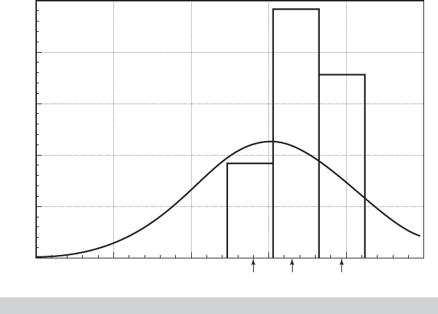
Figure 17.3 shows the implied distribution for the coefﬁcient on age. For the continuous

distribution, we have simply plotted the normal density. For the discrete distribution, we ﬁrst

obtained the mean (0.0358) and standard deviation (0.0107). Notice that the distribution is

tighter than the estimated continuous normal (mean, 0.026, standard deviation, 0.0253). To

suggest the variation of the parameter (purely for purpose of the display, because the distri-

bution is discrete), we placed the mass of the center interval, 0.462, between the midpoints of

the intervals between the center mass point and the two extremes. With a width of 0.0145 the

density is 0.461 / 0.0145 = 31.8. We used the same interval widths for the outer segments.

This range of variation covers about ﬁve standard deviations of the distribution.

17.4.9 NONRESPONSE, ATTRITION, AND INVERSE PROBABILITY

WEIGHTING

Missing observations is a common problem in the analysis of panel data. Nicoletti and

Peracchi (2005) suggest several reasons that, for example, panels become unbalanced:

•

Demographic events such as death;

•

Movement out of the scope of the survey, such as institutionalization or emigration;

We have arrived (once again) at a point where the question of replicability arises. Nonreplicability is

an ongoing challenge in empirical work in economics. (See, for example, Example 17.12.) The problem is

particularly acute in analyses that involve simulation such as Monte Carlo studies and random parameter

models. In the interest of replicability, we note that the random parameter estimates in Table 17.14 were

computed with NLOGIT [Econometric Software (2007)] and are based on 50 Halton draws. We used the ﬁrst

six sequences (prime numbers 2, 3, 5, 7, 11, 13) and discarded the ﬁrst 10 draws in each sequence.

CHAPTER 17

✦

Discrete Choice

735

0.0250.050

0.000

B_INCOME

Density

0.25 0.0750.050

FIGURE 17.3

Distributions of Income Coefﬁcient.

•

Refusal to respond at subsequent waves;

•

Absence of the person at the address;

•

Other types of noncontact.

The GSOEP that we (from Riphahn, Wambach, and Million (2003)) have used in many

examples in this text is one such data set. Jones, Koolman, and Rice (2006) (JKR)

list several other applications, including the British Household Panel Survey (BHPS),

the European Community Household Panel (ECHP), and the Panel Study of Income

Dynamics (PSID).

If observations are missing completely at random (MCAR, see Section 4.7.4) then

the problem of nonresponse can be ignored, though for estimation of dynamic mod-

els, either the analysis will have to be restricted to observations with uninterrupted

sequences of observations, or some very strong assumptions and interpolation methods

will have to be employed to ﬁll the gaps. (See Section 4.7.4 for discussion of the termi-

nology and issues in handling missing data.) The problem for estimation arises when

observations are missing for reasons that are related to the outcome variable of interest.

Nonresponse bias and a related problem, attrition bias (individuals leave permanently

during the study) result when conventional estimators, such as least squares or the pro-

bit maximum likelihood estimator being used here, are applied to samples in which

observations are present or absent from the sample for reasons related to the outcome

variable. It is a form of sample selection bias, that we will examine further in Chapter 19.

Verbeek and Nijman (1992) have suggested a test for endogeneity of the sample

response pattern. (We will adopt JKR’s notation and terminology for this.) Let h denote

the outcome of interest and x denote the relevant set of covariates. Let R denote the

pattern of response. If nonresponse is (completely) random, then E[h |x, R] = E[h |x].

This suggests a variable addition test (neglecting other panel data effects); a pooled

736

PART IV

✦

Cross Sections, Panel Data, and Microeconometrics

model that contains R in addition to x can provide the means for a simple test of

endogeneity. JKR (and Verbeek and Nijman) suggest using the number of waves at

which the individual is present as the measure of R. Thus, adding R to the pooled

model, we can use a simple t test for the hypothesis.

Devising an estimator given that (non)response is nonignorable requires a more

detailed understanding of the process generating the response pattern. The crucial

issue is whether the sample selection is based “on unobservables” or “on observables.”

Selection on unobservables results when, after conditioning on the relevant variables,

x and other information, z, the sampling mechanism is still nonrandom with respect to

the disturbances in the models. Selection on unobservables is at the heart of the sample

selectivity methodology pioneered by Heckman (1979) that we will study in Chapter 19.

(Some applications of the role of unobservables in biased estimation are discussed in

Chapter 8, where we examine sources of endogeneity in regression models.) If selection

is on observables and then conditioned on an appropriate speciﬁcation involving the

observable information, (x,z), a consistent estimator of the model parameters will be

available by “purging” the estimator of the endogeneity of the sampling mechanism.

JKR adopt an inverse probability weighted (IPW) estimator devised by Robins,

Rotnitsky and Zhao (1995), Fitzgerald, Gottshalk, and Mofﬁtt (1998), Mofﬁtt, Fitzger-

ald and Gottshalk (1999), and Wooldridge (2002). The estimator is based on the general

MCAR assumption that P(R = 1 |h, x, z) = P(R = 1 |x, z). That is, the observable

covariates convey all the information that determines the response pattern—the prob-

ability of nonresponse does not vary systematically with the outcome variable once the

exogenous information is accounted for. Implementing this idea in an estimator would

require that x and z be observable when R = 0, that is, the exogenous data be avail-

able for the nonresponders. This will typically not be the case; in an unbalanced panel,

the entire observation is missing. Wooldridge (2002) proposed a somewhat stronger

assumption that makes estimation feasible: P(R = 1 |h, x, z) = P(R = 1 |z) where z is

a set of covariates available at wave 1 (entry to the study). To compute Wooldridge’s

IPW estimator, we will begin with the sample of all individuals who are present at wave

1 of the study. (In our Example 17.17, based on the GSOEP data, not all individuals

are present at the ﬁrst wave.) At wave 1, (x

, z

) are observed for all individuals to be

studied; z

contains information on observables that are not included in the outcome

equation and that predict the response pattern at subsequent waves, including the re-

sponse variable at the ﬁrst wave. At wave 1, then, P(R

= 1 |x

, z

) = 1. Wooldridge

suggests using a probit model for P(R

= 1 |x

, z

), t = 2,...,T for the remain-

ing waves to obtain predicted probabilities of response, ˆp

. The IPW estimator then

maximizes the weighted log likelihood

ln L

IPW



i=1



t=1

ˆp

ln L

Inference based on the weighted log-likelihood function can proceed as in Section 17.3.

A remaining detail concerns whether the use of the predicted probabilities in the

weighted log-likelihood function makes it necessary to correct the standard errors for

two-step estimation. The case here is not an application of the two-step estimators we

considered in Section 14.7, since the ﬁrst step is not used to produce an estimated param-

eter vector in the second. Wooldridge (2002) shows that the standard errors computed

CHAPTER 17

✦

Discrete Choice

737

2134

NUM_WAVE

567

976

732

488

Frequency

244

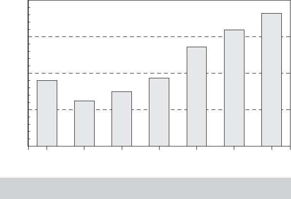
FIGURE 17.4

Number of Waves Responded for Those Present at

Wave

without the adjustment are “conservative” in that they are larger than they would be

with the adjustment.

Example 17.17 Nonresponse in the GSOEP Sample

Of the 7,293 individuals in the GSOEP data that we have used in several earlier examples,

3,874 were present at wave 1 (1984) of the sample. The pattern of the number of waves

present by these 3,874 is shown in Figure 17.4. The waves are 1984–1988, 1991, and 1994.

A dynamic model would be based on the 1,600 of those present at wave 1 who were also

present for the next four waves. There is a substantial amount of nonresponse in these data.

Not all individuals exit the sample with the ﬁrst nonresponse, however, so the resulting panel

remains unbalanced. The impression suggested by Figure 17.4 could be a bit misleading—

the nonresponse pattern is quite different from simple attrition. For example, of the 3,874

individuals who responded at wave 1, 364 did not respond at wave 2 but returned to the

sample at wave 3.

To employ the Verbeek and Nijman test, we used the entire sample of 27,326 household

years of data. The pooled probit model for DocVis > 0 produced the results at the left in

Table 17.14. A t (Wald) test of the hypothesis that the coefﬁcient on number of waves present

is zero is strongly rejected, so we proceed to the inverse probability weighted estimator. For

computing the inverse probability weights, we used the following speciﬁcation:

i 1

= constant, age, income, educ, kids, married

i 1

= female, handicapped dummy, percentage handicapped,

university, working, blue collar, white collar, public servant, y

i 1

= Doctor Visits > 0 in period 1.

This ﬁrst-year data vector is used as the observed explanatory variables in probit models for

waves 2–7 for the 3,874 individuals who were present at wave 1. There are 3,874 observations

for each of these probit models, since all were observed at wave 1. Fitted probabilities for R

are computed for waves 2–7, while R

i 1

= 1. The sample means of these probabilities which

equals the proportion of the 3,874 who responded at each wave are 1.000, 0.730, 0.672,

0.626, 0.682, 0.568, and 0.386, respectively. Table 17.14 presents the estimated models for

several speciﬁcations In each case, it appears that the weighting brings some moderate

changes in the parameters and, uniformly, reductions in the standard errors.

738

PART IV

✦

Cross Sections, Panel Data, and Microeconometrics

TABLE 17.14

Inverse Probability Weighted Estimators

Random Effects—

Pooled Model Mundlak Fixed Effects

Variable Endog. Test Unwtd. IPW Unwtd. IPW Unwtd. IPW

Constant 0.26411 0.03369 −0.02373 0.09838 0.13237

(0.05893) (0.07684) (0.06385) (0.16081) (0.17019)

Age 0.01369 0.01667 0.01831 0.05141 0.05656 0.06210 0.06841

(0.00080) (0.00107) (0.00088) (0.00422) (0.00388) (0.00506) (0.00465)

Income −0.12446 −0.17097 −0.22263 0.05794 0.01699 0.07880 0.03603

(0.04636) (0.05981) (0.04801) (0.11256) (0.10580) (0.12891) (0.12193)

Education −0.02925 −0.03614 −0.03513 −0.06456 −0.07058 −0.07752 −0.08574

(0.00351) (0.00449) (0.00365) (0.06104) (0.05792) (0.06582) (0.06149)

Kids −0.13130 −0.13077 −0.13277 −0.04961 −0.03427 −0.05776 −0.03546

(0.01828) (0.02303) (0.01950) (0.04500) (0.04356) (0.05296) (0.05166)

Married 0.06759 0.06237 0.07015 −0.06582 −0.09235 −0.07939 −0.11283

(0.02060) (0.02616) (0.02097) (0.06596) (0.06330) (0.08146) (0.07838)

Mean Age −0.03056 −0.03401

(0.00479) (0.00455)

Mean Income −0.66388 −0.78077

(0.18646) (0.18866)

Mean 0.02656 0.02899

Education (0.06160) (0.05848)

Mean Kids −0.17524 −0.20615

(0.07266) (0.07464)

Mean Married 0.22346 0.25763

(0.08719) (0.08433)

Number −0.02977

of Waves (0.00450)

ρ 0.46538 0.48616

17.5 BIVARIATE AND MULTIVARIATE PROBIT

MODELS

In Chapter 10, we analyzed a number of different multiple-equation extensions of the

classical and generalized regression model. A natural extension of the probit model

would be to allow more than one equation, with correlated disturbances, in the same

spirit as the seemingly unrelated regressions model. The general speciﬁcation for a

two-equation model would be

∗

= x



+ ε

, y

= 1ify

∗

> 0, 0 otherwise,

∗

= x



+ ε

, y

= 1ify

∗

> 0, 0 otherwise,



, x



∼ N







1 ρ

ρ 1



(17-48)

This bivariate probit model is interesting in its own right for modeling the joint deter-

mination of two variables, such as doctor and hospital visits in the next example. It also

provides the framework for modeling in two common applications. In many cases, a

treatment effect, or endogenous inﬂuence, takes place in a binary choice context. The

bivariate probit model provides a speciﬁcation for analyzing a case in which a probit