Greene W.H. Econometric Analysis

Подождите немного. Документ загружается.

CHAPTER 18

✦

Discrete Choices and Event Counts

789

probabilities are

Prob(y = 0 |x) = 1 −(x



β),

Prob(y = 1 |x) = (μ −x



β) − (−x



β),

Prob(y = 2 |x) = 1 −(μ − x



β).

For the three probabilities, the partial effects of changes in the regressors are

∂ Prob(y = 0 |x)

∂x

=−φ(x



β)β,

∂ Prob(y = 1 |x)

∂x

= [φ(−x



β) − φ(μ − x



β)]β,

∂ Prob(y = 2 |x)

∂x

= φ(μ − x



β)β.

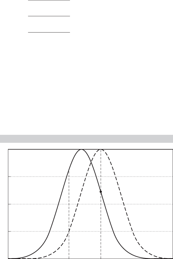
Figure 18.4 illustrates the effect. The probability distributions of y and y

∗

are shown in

the solid curve. Increasing one of the x’s while holding β and μ constant is equivalent

to shifting the distribution slightly to the right, which is shown as the dashed curve.

The effect of the shift is unambiguously to shift some mass out of the leftmost cell.

Assuming that β is positive (for this x), Prob(y = 0 |x) must decline. Alternatively,

from the previous expression, it is obvious that the derivative of Prob(y = 0 |x) has the

opposite sign from β. By a similar logic, the change in Prob(y = 2 |x) [or Prob(y = J |x)

in the general case] must have the same sign as β. Assuming that the particular β is

positive, we are shifting some probability into the rightmost cell. But what happens

to the middle cell is ambiguous. It depends on the two densities. In the general case,

relative to the signs of the coefﬁcients, only the signs of the changes in Prob(y = 0 |x)

and Prob(y = J |x) are unambiguous! The upshot is that we must be very careful

FIGURE 18.4

Effects of Change in

on Predicted Probabilities.

102

0.1

0.2

0.3

0.4

790

PART IV

✦

Cross Sections, Panel Data, and Microeconometrics

in interpreting the coefﬁcients in this model. Indeed, without a fair amount of extra

calculation, it is quite unclear how the coefﬁcients in the ordered probit model should

be interpreted.

Example 18.3 Rating Assignments

Marcus and Greene (1985) estimated an ordered probit model for the job assignments of

new Navy recruits. The Navy attempts to direct recruits into job classiﬁcations in which they

will be most productive. The broad classiﬁcations the authors analyzed were technical jobs

with three clearly ranked skill ratings: “medium skilled,” “highly skilled,” and “nuclear quali-

ﬁed/highly skilled.” Because the assignment is partly based on the Navy’s own assessment

and needs and partly on factors speciﬁc to the individual, an ordered probit model was

used with the following determinants: (1) ENSPE = a dummy variable indicating that the

individual entered the Navy with an “A school” (technical training) guarantee; (2) EDMA =

educational level of the entrant’s mother; (3) AFQT = score on the Armed Forces Qualifying

Test; (4) EDYRS =years of education completed by the trainee; (5) MARR =a dummy variable

indicating that the individual was married at the time of enlistment; and (6) AGEAT = trainee’s

age at the time of enlistment. (The data used in this study are not available for distribution.)

The sample size was 5,641. The results are reported in Table 18.10. The extremely large t

ratio on the AFQT score is to be expected, as it is a primary sorting device used to assign

job classiﬁcations.

To obtain the marginal effects of the continuous variables, we require the standard normal

density evaluated at −¯x



β =−0.8479 and ˆμ − ¯x



β = 0.9421. The predicted probabilities are

(−0.8479) = 0.198, (0.9421) − (−0.8479) = 0.628, and 1 − (0.9421) = 0.174. ( The

actual frequencies were 0.25, 0.52, and 0.23.) The two densities are φ ( −0.8479) =0.278 and

φ(0.9421) = 0.255. Therefore, the derivatives of the three probabilities with respect to AFQT,

for example, are

∂ P

∂AFQT

= (−0.278) 0.039 =−0.01084,

∂ P

∂AFQT

= (0.278 − 0.255) 0.039 = 0.0009,

∂ P

∂AFQT

= 0.255(0.039) = 0.00995.

Note that the marginal effects sum to zero, which follows from the requirement that the

probabilities add to one. This approach is not appropriate for evaluating the effect of a dummy

variable. We can analyze a dummy variable by comparing the probabilities that result when

the variable takes its two different values with those that occur with the other variables held

at their sample means. For example, for the MARR variable, we have the results given in

Table 18.11.

TABLE 18.10

Estimated Rating

Assignment Equation

Mean of

Variable Estimate t Ratio Variable

Constant −4.34 — —

ENSPA 0.057 1.7 0.66

EDMA 0.007 0.8 12.1

AFQT 0.039 39.9 71.2

EDYRS 0.190 8.7 12.1

MARR −0.48 −9.0 0.08

AGEAT 0.0015 0.1 18.8

μ 1.79 80.8 —

CHAPTER 18

✦

Discrete Choices and Event Counts

791

TABLE 18.11

Marginal Effect of a Binary Variable

−



xˆμ −



x Prob[y = 0] Prob[y = 1] Prob[y = 2]

MARR = 0 −0.8863 0.9037 0.187 0.629 0.184

MARR = 1 −0.4063 1.3837 0.342 0.574 0.084

Change 0.155 −0.055 −0.100

18.3.2 A SPECIFICATION TEST FOR THE ORDERED CHOICE

MODEL

The basic formulation of the ordered choice model implies that for constructed binary

variables,

= 1ify

≤ j, 0 otherwise, j = 1, 2,..., J − 1, (18-16)

Prob(w

= 1 |x

) = F(x



β−μ

The ﬁrst of these, when j = 1, is the binary choice model of Section 17.2. One implication

is that we could estimate the slopes, but not the threshold parameters, in the ordered

choice model just by using w

and x

in a binary probit or logit model. (Note that this

result also implies the validity of combining adjacent cells in the ordered choice model.)

But, (18-16) also deﬁnes a set of J −1 binary choice models with different constants but

common slope vector, β. This equality of the parameter vectors in (18-16) has been

labeled the parallel regression assumption. Although it is merely an implication of the

model speciﬁcation, this has been viewed as an implicit restriction on the model. [See,

for example, Long (1997, p. 141).] Brant (1990) suggests a test of the parallel regressions

assumption based on (18-16). One can, in principle, ﬁt J −1 such binary choice models

separately. Each will produce its own constant term and a consistent estimator of the

common β. Brant’s Wald test examines the linear restrictions β

= β

=···=β

J −1

,or

: β

− β

= 0, q = 2,..., J − 1. The Wald statistic will be

[(J − 2)K] = (R

∗

)



[R × Asy.Var[

∗

] × R



]

−1

∗

where

∗

is obtained by stacking the individual binary logit or probit estimates of β

(without the constant terms). [See Brant (1990), Long (1997), or Greene and Hensher

(2010, page 187) for details on computing the statistic.]

Rejection of the null hypothesis calls the model speciﬁcation into question. An

alternative model in which there is a different β for each value of y has two problems:

it does not force the probabilities to be positive and it is internally inconsistent. On the

latter point, consider the suggested latent regression, y

∗

= x



+ε. If the “β” is different

for each j, then it is not possible to construct a data generating mechanism for y

∗

(or,

for example, simulate it); the realized value of y

∗

cannot be deﬁned without knowing

y (that is, the realized j), since the applicable β depends on j, but y is supposed to be

determined from y

∗

through, for example, (18-16). There is no parametric restriction

other than the one we seek to avoid that will preserve the ordering of the probabilities

for all values of the data and maintain the coherency of the model. This still leaves

the question of what speciﬁcation failure would logically explain the ﬁnding. Some

suggestions in Brant (1990) include (1) misspeciﬁcation of the latent regression, x



β;

792

PART IV

✦

Cross Sections, Panel Data, and Microeconometrics

(2) heteroscedasticity of ε; and (3) misspeciﬁcation of the distributional form for the

latent variable, that is, “nonlogistic link function.”

Example 18.4 Brant Test for an Ordered Probit Model of Health

Satisfaction

In Example 17.4, we studied the health care usage of a sample of households in the

German Socioeconomic Panel (GSOEP). The data include a self-reported measure of “health

satisfaction,” (HSAT) that is coded 0–10. This variable provides a natural application of the

ordered choice models in this chapter. The data are an unbalanced panel. For purposes of

this exercise, we have used the ﬁfth (1984) wave of the data set, which is a cross section of

4,483 observations. We then collapsed the 10 cells into 5 [(0–2),(3–5), (6–8),(9),(10)] for this

example. The utility function is

HSAT

∗

= β

+ β

AGE

+ β

INCOME

+ β

KIDS

+ β

EDUC

+ β

MARRIED

WORKING

+ ε

Variables KIDS, MARRIED, and WORKING, are binary indicators of whether there are children

in the household, marital status, and whether the individual was working at the time of the

survey. (These data are examined further in Example 18.6.) The model contains six variables,

and there are four binary choice models ﬁt, so there are ( J −2) ( K ) = (3)(6) = 18 restrictions.

The chi-squared for the probit model is 87.836. The critical value for 95 percent is 28.87, so

the homogeneity restriction is rejected. The corresponding value for the logit model is 77.84,

which leads to the same conclusion.

18.3.3 BIVARIATE ORDERED PROBIT MODELS

There are several extensions of the ordered probit model that follow the logic of the

bivariate probit model we examined in Section 17.5. A direct analog to the base case

two-equation model is used in the study in Example 18.5.

Example 18.5 Calculus and Intermediate Economics Courses

Butler et al. (1994) analyzed the relationship between the level of calculus attained and

grades in intermediate economics courses for a sample of Vanderbilt students. The two-step

estimation approach involved the following strategy. (We are stylizing the precise formulation

a bit to compress the description.) Step 1 involved a direct application of the ordered probit

model of Section 18.3.1 to the level of calculus achievement, which is coded 0, 1, ...,6:

∗

= x



β + ε

, ε

∼ N[0, 1],

= 0if −∞ < m

∗

≤ 0

= 1if0< m

∗

≤ μ

···

= 6ifμ

< m

∗

< +∞.

The authors argued that although the various calculus courses can be ordered discretely

by the material covered, the differences between the levels cannot be measured directly.

Thus, this is an application of the ordered probit model. The independent variables in this

ﬁrst-step model included SAT scores, foreign language proﬁciency, indicators of intended

major, and several other variables related to areas of study.

The second step of the estimator involves regression analysis of the grade in the interme-

diate microeconomics or macroeconomics course. Grades in these courses were translated

to a granular continuous scale (A = 4.0, A−=3.7, etc.). A linear regression is speciﬁed,

Grade

= z



δ + u

, where u

∼ N



0, σ



CHAPTER 18

✦

Discrete Choices and Event Counts

793

Independent variables in this regression include, among others, (1) dummy variables for

which outcome in the ordered probit model applies to the student (with the zero reference

case omitted), (2) grade in the last calculus course, (3) several other variables related to

prior courses, (4) class size, (5) freshman GPA, and so on. The unobservables in the Grade

equation and the math attainment are clearly correlated, a feature captured by the additional

assumption that (ε

, u

, z

) ∼ N

[(0, 0) , (1, σ

),ρσ

]. A nonzero ρ captures this “selection”

effect. With this in place, the dummy variables in (1) have now become endogenous. The

solution is a “selection” correction that we will examine in detail in Chapter 19. The modiﬁed

equation becomes

Grade

= z



δ + E[u

] + v

= z



δ + ( ρσ

)[λ(x



β, μ

, ..., μ

)]+ v

They thus adopt a “control function” approach to accommodate the endogeneity of the math

attainment dummy variables. [See Section 17.3.5 and (17-32) for another application of this

method.] The term λ(x



β, μ

, ..., μ

) is a generalized residual that is constructed using the

estimates from the ﬁrst-stage ordered probit model. [A precise statement of the form of this

variable is given in Li and Tobias (2006).] Linear regression of the course grade on z

and this

constructed regressor is computed at the second step. The standard errors at the second

step must be corrected for the use of the estimated regressor using what amounts to a

Murphy and Topel (2002) correction. (See Section 14.7.)

Li and Tobias (2006) in a replication of and comment on Butler et al. (1994), after roughly

replicating the classical estimation results with a Bayesian estimator, observe that the pre-

ceding Grade equation above could also be treated as an ordered probit model. The resulting

bivariate ordered probit model would be

∗

= x



β + ε

, and g

∗

= z



δ + u

= 0if−∞ < m

∗

≤ 0 g

= 0if−∞ < g

∗

≤ 0

= 1if0< m

∗

≤ μ

= 1if0< g

∗

≤ α

··· ···

= 6ifμ

< m

∗

< +∞. = 11 if μ

< g

∗

< +∞

where

(ε

, u

, z

) ∼ N



(0,0),



1, σ



, ρσ



Li and Tobias extended their analysis to this case simply by “transforming” the dependent

variable in Butler et al.’s second equation. Computing the log-likelihood using sets of bi-

variate normal probabilities is fairly straightforward for the bivariate ordered probit model.

[See Greene (2007).] However, the classical study of these data using the bivariate ordered

approach remains to be done, so a side-by-side comparison to Li and Tobias’s Bayesian

alternative estimator is not possible. The endogeneity of the calculus dummy variables

in (1) remains a feature of the model, so both the MLE and the Bayesian posterior

are less straightforward than they might appears. Whether the results in Section 17.5.5

on the recursive bivariate probit model extend to this case also remains to be

determined.

The bivariate ordered probit model has been applied in a number of settings in the

recent empirical literature, including husband and wife’s education levels [Magee et al.

(2000)], family size [(Calhoun (1991)], and many others. In two early contributions to

the ﬁeld of pet econometrics, Butler and Chatterjee analyze ownership of cats and dogs

(1995) and dogs and televisions (1997).

794

PART IV

✦

Cross Sections, Panel Data, and Microeconometrics

18.3.4 PANEL DATA APPLICATIONS

The ordered probit model is used to model discrete scales that represent indicators

of a continuous underlying variable such as strength of preference, performance, or

level of attainment. Many of the recently assembled national panel data sets con-

tain survey questions that ask about subjective assessments of health, satisfaction, or

well-being, all of which are applications of this interpretation. Examples include the

following:

•

The European Community Household Panel (ECHP) includes questions about job

satisfaction [see D’Addio (2004)].

•

The British Household Panel Survey (BHPS) includes questions about health status

[see Contoyannis et al. (2004)].

•

The German Socioeconomic Household Panel (GSOEP) includes questions about

subjective well-being [see Winkelmann (2004)] and subjective assessment of health

satisfaction [see Riphahn et al. (2003) and Example 18.4].

Ostensibly, the applications would ﬁt well into the ordered probit frameworks already

described. However, given the panel nature of the data, it will be desirable to augment

the model with some accommodation of the individual heterogeneity that is likely to

be present. The two standard models, ﬁxed and random effects, have both been applied

to the analyses of these survey data.

18.3.4.a Ordered Probit Models with Fixed Effects

D’Addio et al. (2003), using methodology developed by Frijters et al. (2004) and Ferrer-

i-Carbonel et al. (2004), analyzed survey data on job satisfaction using the Danish

component of the European Community Household Panel. Their estimator for an or-

dered logit model is built around the logic of Chamberlain’s estimator for the binary

logit model. [See Section 17.4.4.] Because the approach is robust to individual speciﬁc

threshold parameters and allows time-invariant variables, it differs sharply from the

ﬁxed effects models we have considered thus far as well as from the ordered probit

model of Section 18.3.1.

Unlike Chamberlain’s estimator for the binary logit model,

however, their conditional estimator is not a function of minimal sufﬁcient statistics. As

such, the incidental parameters problem remains an issue.

Das and van Soest (2000) proposed a somewhat simpler approach. [See, as well,

Long’s (1997) discussion of the “parallel regressions assumption,” which employs this

device in a cross-section framework.] Consider the base case ordered logit model with

ﬁxed effects,

∗

= α

+ x



β + ε

,ε

∼ N[0, 1],

= j if μ

j−1

< y

∗

<μ

, j = 0, 1,...,J and μ

−1

=−∞,μ

= 0,μ

=+∞.

The model assumptions imply that

Prob(y

= j |X

) = (μ

− α

− x



β) − (μ

j−1

− α

− x



β),

Cross-section versions of the ordered probit model with individual speciﬁc thresholds appear in Terza

(1985a), Pudney and Shields (2000), and Greene (2007).

CHAPTER 18

✦

Discrete Choices and Event Counts

795

where (t) is the cdf of the logistic distribution. Now, deﬁne a binary variable

it, j

= 1ify

> j, j = 0,..., J − 1.

It follows that

Prob[w

it, j

= 1 |X

] = (α

− μ

+ x



β)

= (θ

+ x



β).

The “ j ” speciﬁc constant, which is the same for all individuals, is absorbed in θ

. Thus,

a ﬁxed effects binary logit model applies to each of the J − 1 binary random variables,

it, j

. The method in Section 17.4.4 can now be applied to each of the J − 1 random

samples. This provides J −1 estimators of the parameter vector β (but no estimator of

the threshold parameters). The authors propose to reconcile these different estimators

by using a minimum distance estimator of the common true β. (See Section 13.3.) The

minimum distance estimator at the second step is chosen to minimize

q =

J −1



j=0

J −1



m=0

(

− β)





−1



(

− β),

where [V

−1

] is the j, m block of the inverse of the ( J − 1)K × (J − 1)K partitioned

matrix V that contains Asy. Cov[

]. The appropriate form of this matrix for a set

of cross-section estimators is given in Brant (1990). Das and van Soest (2000) used the

counterpart for Chamberlain’s ﬁxed effects estimator but do not provide the speciﬁcs

for computing the off-diagonal blocks in V.

The full ordered probit model with ﬁxed effects, including the individual speciﬁc

constants, can be estimated by unconditional maximum likelihood using the results in

Section 14.9.6.d. The likelihood function is concave [see Pratt (1981)], so despite its

superﬁcial complexity, the estimation is straightforward. (In the following application,

with more than 27,000 observations and 7,293 individual effects, estimation of the full

model required roughly ﬁve seconds of computation.) No theoretical counterpart to

the Hsiao (1986, 2003) and Abrevaya (1997) results on the small T bias (incidental

parameters problem) of the MLE in the presence of ﬁxed effects has been derived

for the ordered probit model. The Monte Carlo results in Greene (2004) (see, as well,

Section 15.5.2), suggest that biases comparable to those in the binary choice models

persist in the ordered probit model as well. As in the binary choice case, the complication

of the ﬁxed effects model is the small sample bias, not the computation. The Das and

van Soest approach ﬁnesses this problem—their estimator is consistent—but at the cost

of losing the information needed to compute partial effects or predicted probabilities.

18.3.4.b Ordered Probit Models with Random Effects

The random effects ordered probit model model has been much more widely used than

the ﬁxed effects model. Applications include Groot and van den Brink (2003), who stud-

ied training levels of employees, with ﬁrm effects; Winkelmann (2003b), who examined

subjective measures of well-being with individual and family effects; Contoyannis et al.

(2004), who analyzed self-reported measures of health status; and numerous others.

In the simplest case, the method of the Butler and Mofﬁtt (1982) quadrature method

(Section 14.9.6.c) can be extended to this model.

796

PART IV

✦

Cross Sections, Panel Data, and Microeconometrics

Example 18.6 Health Satisfaction

The GSOEP German Health Care data that we have used in Examples 11.16, 17.4, and others

includes a self-reported measure of health satisfaction, HSAT, that takes values 0, 1, ..., 10.

This is a typical application of a scale variable that reﬂects an underlying continuous variable,

“health.” The frequencies and sample proportions for the reported values are as follows:

HSAT Frequency Proportion

0 447 1.6%

1 255 0.9%

2 642 2.3%

3 1,173 4.2%

4 1,390 5.0%

5 4,233 15.4%

6 2,530 9.2%

7 4,231 15.4%

8 6,172 22.5%

9 3,061 11.2%

10 3,192 11.6%

We have ﬁt pooled and panel data versions of the ordered probit model to these data. The

model used is

∗

= β

+β

Age

+β

Income

+β

Kids

Education

+β

Married

+β

Working

+ε

where c

will be the common ﬁxed or random effect. (We are interested in comparing the ﬁxed

and random effects estimators, so we have not included any time-invariant variables such

as gender in the equation.) Table 18.12 lists ﬁve estimated models. (Standard errors for the

estimated threshold parameters are omitted.) The ﬁrst is the pooled ordered probit model. The

second and third are ﬁxed effects. Column 2 shows the unconditional ﬁxed effects estimates

using the results of Section 14.9.6.d. Column 3 shows the Das and van Soest estimator. For

the minimum distance estimator, we used an inefﬁcient weighting matrix, the block-diagonal

matrix in which the j th block is the inverse of the j th asymptotic covariance matrix for the

individual logit estimators. With this weighting matrix, the estimator is

MDE





j =0

−1



−1



j =0

−1

and the estimator of the asymptotic covariance matrix is approximately equal to the bracketed

inverse matrix. The fourth set of results is the random effects estimator computed using

the maximum simulated likelihood method. This model can be estimated using Butler and

Mofﬁtt’s quadrature method; however, we found that even with a large number of nodes,

the quadrature estimator converged to a point where the log-likelihood was far lower than

the MSL estimator, and at parameter values that were implausibly different from the other

estimates. Using different starting values and different numbers of quadrature points did not

change this outcome. The MSL estimator for a random constant term (see Section 15.6.3)

is considerably slower but produces more reasonable results. The ﬁfth set of results is the

Mundlak form of the random effects model, which includes the group means in the models

as controls to accommodate possible correlation between the latent heterogeneity and the

included variables. As noted in Example 18.3, the components of the ordered choice model

must be interpreted with some care. By construction, the partial effects of the variables on

In the original data set, 40 (of 27,326) observations on this variable were coded with noninteger values

between 6 and 7. For purposes of our example, we have recoded all 40 observations to 7.

CHAPTER 18

✦

Discrete Choices and Event Counts

797

TABLE 18.12

Estimated Ordered Probit Models for Health Satisfaction

(5)

(2) (3) (4) Random Effects

Mundlak Controls

(1) Fixed Effects Fixed Effects Random

Variable Pooled Unconditional Conditional Effects Variables Means

Constant 2.4739 3.8577 3.2603

(0.04669) (0.05072) (0.05323)

Age −0.01913 −0.07162 −0.1011 −0.03319 −0.06282 0.03940

(0.00064) (0.002743) (0.002878) (0.00065) (0.00234) (0.002442)

Income 0.1811 0.2992 0.4353 0.09436 0.2618 0.1461

(0.03774) (0.07058) (0.07462) (0.03632) (0.06156) (0.07695)

Kids 0.06081 −0.06385 −0.1170 0.01410 −0.05458 0.1854

(0.01459) (0.02837) (0.03041) (0.01421) (0.02566) (0.03129)

Education 0.03421 0.02590 0.06013 0.04728 0.02296 0.02257

(0.002828) (0.02677) (0.02819) (0.002863) (0.02793) (0.02807)

Married 0.02574 0.05157 0.08505 0.07327 0.04605 −0.04829

(0.01623) (0.04030) (0.04181) (0.01575) (0.03506) (0.03963)

Working 0.1292 −0.02659 −0.007969 0.07108 −0.02383 0.2702

(0.01403) (0.02758) (0.02830) (0.01338) (0.02311) (0.02856)

0.1949 0.3249 0.2726 0.2752

0.5029 0.8449 0.7060 0.7119

0.8411 1.3940 1.1778 1.1867

1.111 1.8230 1.5512 1.5623

1.6700 2.6992 2.3244 2.3379

1.9350 3.1272 2.6957 2.7097

2.3468 3.7923 3.2757 3.2911

3.0023 4.8436 4.1967 4.2168

3.4615 5.5727 4.8308 4.8569

0.0000 0.0000 1.0078 0.9936

ln L −56,813.52 −41,875.63 −53,215.54 −53,070.43

TABLE 18.13

Estimated Marginal Effects: Pooled Model

HSAT Age Income Kids Education Married Working

0 0.0006 −0.0061 −0.0020 −0.0012 −0.0009 −0.0046

1 0.0003 −0.0031 −0.0010 −0.0006 −0.0004 −0.0023

2 0.0008 −0.0072 −0.0024 −0.0014 −0.0010 −0.0053

3 0.0012 −0.0113 −0.0038 −0.0021 −0.0016 −0.0083

4 0.0012 −0.0111 −0.0037 −0.0021 −0.0016

−0.0080

5 0.0024 −0.0231 −0.0078 −0.0044 −0.0033 −0.0163

6 0.0008 −0.0073 −0.0025 −0.0014 −0.0010 −0.0050

7 0.0003 −0.0024 −0.0009 −0.0005 −0.0003 −0.0012

8 −0.0019 0.0184 0.0061 0.0035 0.0026 0.0136

9 −0.0021 0.0198 0.0066 0.0037 0.0028 0.0141

10 −0.0035 0.0336 0.0114 0.0063 0.0047 0.0233

the probabilities of the outcomes must change sign, so the simple coefﬁcients do not show

the complete picture implied by the estimated model. Table 18.13 shows the partial effects

for the pooled model to illustrate the computations.

Winkelmann (2003b) used the random effects approach to analyze the subjec-

tive well-being (SWB) question (also coded 0 to 10) in the German Socioeconomic

798

PART IV

✦

Cross Sections, Panel Data, and Microeconometrics

Panel (GSOEP) data set. The ordered probit model in this study is based on the latent

regression

∗

imt

= x



imt

β + ε

imt

+ u

+ v

The independent variables include age, gender, employment status, income, family size,

and an indicator for good health. An unusual feature of the model is the nested random

effects (see Section 14.9.6.b), which include a family effect, v

, as well as the individual

family member (i in family m) effect, u

. The GLS/MLE approach we applied to

the linear regression model in Section 14.9.6.b is unavailable in this nonlinear setting.

Winkelmann instead employed a Hermite quadrature procedure to maximize the log-

likelihood function.

Contoyannis, Jones, and Rice (2004) analyzed a self-assessed health scale that

ranged from 1 (very poor) to 5 (excellent) in the British Household Panel Survey. Their

model accommodated a variety of complications in survey data. The latent regression

underlying their ordered probit model is

∗

= x



β + H



i,t−1

γ + α

+ ε

where x

includes marital status, race, education, household size, age, income, and num-

ber of children in the household. The lagged value, H

i,t−1

, is a set of binary variables

for the observed health status in the previous period. (This is the same device that was

used by Butler et al. in Example 18.5.) In this case, the lagged values capture state

dependence—the assumption that the health outcome is redrawn randomly in each

period is inconsistent with evident runs in the data. The initial formulation of the re-

gression is a ﬁxed effects model. To control for the possible correlation between the

effects, α

, and the regressors, and the initial conditions problem that helps to explain

the state dependence, they use a hybrid of Mundlak’s (1978) correction and a suggestion

by Wooldridge (2002a) for modeling the initial conditions,

= α



+ H



i,1

δ + u

where u

is exogenous. Inserting the second equation into the ﬁrst produces a random

effects model that can be ﬁt using the quadrature method we considered earlier.

18.3.5 EXTENSIONS OF THE ORDERED PROBIT MODEL

The basic speciﬁcation of the ordered probit model can be extended in the same direc-

tions as we considered in constructing models for binary choice in Chapter 17. These

include heteroscedasticity in the random utility function [see Section 17.3.7.b, Keele

and Park (2005), and Wang and Kockelman (2005), for an application] and heterogene-

ity in the preferences (i.e., random parameters and latent classes). [An extensive study

of heterogeneity in health satisfaction based on 22 waves of the GSOEP is Jones and

Schurer (2010).] Two speciﬁcation issues that are speciﬁc to the ordered choice model

are accommodating heterogeneity in the threshold parameters and reconciling differ-

ences in the meaning of the preference scale across different groups. We will sketch

the model extensions in this section. Further details are given in Chapters 6 and 7 of

Hensher and Greene (2010).