Greene W.H. Econometric Analysis

Подождите немного. Документ загружается.

CHAPTER 18

✦

Discrete Choices and Event Counts

779

the disturbances instead of the extreme value assumed in the logit model. In this case,

the scaling of the utility functions is different by a factor of (π

/6)

1/2

= 1.283, as the

probit model assumes ε

has a standard deviation of 1.0.

We also ﬁt three variants of the random parameters logit. In these cases, the choice-

speciﬁc variance for each utility function is σ

+ θ

where σ

is the contribution of the

logit model, which is π

/ 6 =1.645, and θ

is the estimated constant speciﬁc variance

estimated in the random parameters model. The combined estimated standard devia-

tions are given in the table. The estimates of the speciﬁc parameters, θ

, are given in the

footnotes. The estimated models are (1) unrestricted variation and correlation among

the three intercept parameters—this parallels the general speciﬁcation of the multino-

mial probit model; (2) only the constant terms randomly distributed but uncorrelated,

a model that is parallel to the multinomial probit model with no cross-equation cor-

relation and to the heteroscedastic extreme value model shown in Table 18.7 and (3)

random but uncorrelated parameters. This model is more general than the others but is

somewhat restricted as the parameters are assumed to be uncorrelated. Identiﬁcation

of the correlation matrix is weak in this model—after all, we are attempting to estimate

a6× 6 correlation matrix for all unobserved variables. Only the estimated parameters

are shown in Table 18.9. Estimated standard errors are similar to (although generally

somewhat larger than) those for the basic multinomial logit model.

The standard deviations and correlations shown for the multinomial probit model

are parameters of the distribution of ε

, the overall randomness in the model. The coun-

terparts in the random parameters model apply to the distributions of the parameters.

Thus, the full disturbance in the model in which only the constants are random is

iair

+ u

air

for air, and likewise for train and bus. Likewise, the correlations shown

for the ﬁrst two models are directly comparable, although it should be noted that in the

random parameters model, the disturbances have a distribution that is that of a sum

of an extreme value and a normal variable, while in the probit model, the disturbances

are normally distributed. With these considerations, the “unrestricted” models in each

case are comparable and are, in fact, fairly similar.

None of this discussion suggests a preference for one model or the other. The

likelihood values are not comparable, so a direct test is precluded. Both relax the IIA

assumption, which is a crucial consideration. The random parameters model enjoys

a signiﬁcant practical advantage, as discussed earlier, and also allows a much richer

speciﬁcation of the utility function itself. But, the question still warrants additional

study. Both models are making their way into the applied literature.

18.2.10 ESTIMATING WILLINGNESS TO PAY

One of the standard applications of choice models is to estimate how much consumers

value the attributes of the choices. Recall that we are not able to observe the scale of

the utilities in the choice model. However, we can use the marginal utility of income,

also scaled in the same unobservable way, to effect the valuation. In principle, we could

estimate

WTP = (Marginal Utility of Attribute/σ )/(Marginal Utility of Income/σ )

= (β

attribute

/σ )/(γ

Income

/σ ),

780

PART IV

✦

Cross Sections, Panel Data, and Microeconometrics

where σ is the unknown scaling of the utility functions. Note that σ cancels out of the

ratio. In our application, for example, we might assess how much consumers would be

willing to pay to have shorter waits at the terminal for the public modes of transportation

by using

WTP

time

=−β

(

TTME

/γ

Income

(We use the negative because additional time spent waiting at the terminal provides

disutility, as evidenced by its coefﬁcient’s negative sign.) In settings in which income is

not observed, researchers often use the negative of the coefﬁcient on a cost variable

as a proxy for the marginal utility of income. Standard errors for estimates of WTP

can be computed using the delta method or the method of Krinsky and Robb. (See

Sections 4.4.4 and 15.3.)

In the basic multinomial logit model, the estimator of WTP is a simple ratio of

parameters. In our estimated model in Table 18.3, for example, using the household

income coefﬁcient as the numeraire, the estimate of WTP for a shorter wait at the

terminal is −0.09612/0.01329 = 7.239. The units of measurement must be resolved

in this computation, since terminal time is measured in minutes while the cost is in

$1,000/year. Multiplying this result by $60 minutes/hour and dividing by the equivalent

hourly income of income times 8,760/1,000 gives $49.54 per hour of waiting time. To

compute the estimated asymptotic standard error, for convenience, we ﬁrst rescaled

the terminal time to hours by dividing it by 60 and the income variable to $/hour by

multiplying it by 1,000/8,760. The resulting estimated asymptotic distribution for the

estimators is



(

TTME

ˆγ

HINC



∼ N



−5.76749

0.11639





0.392365 0.00193095

0.00193095 0.00808177



The derivatives of WTP

(

TTME

=−β

(

TTME

/γ

are −1/γ

for β

TTME

and –WTP/γ

for γ

. This provides an estimator of 38.8304 for the standard error. The conﬁdence

interval for this parameter would be −26.56 to +125.63. This seems extremely wide. We

will return to this issue later.

In the mixed logit model, if either of the coefﬁcients in the computation is random,

then the preceding simple computation above will not reveal the heterogeneity in the re-

sult. In many studies of WTP using mixed logit models, it is common to allow the utility

parameter on the attribute (numerator) to be random and treat the numeraire (income

or cost coefﬁcient) as nonrandom. Using our mode choice application, we reﬁt the

model with β

(

TTME,i

= β

(

TTME

+σ

(

TTME

and all other coefﬁcients nonrandom. We then

used the method described in Section 15.10 to estimate E[β

(

TTME,i

, choice

]/γ

estimate the expected WTP for each individual in the sample. Income and terminal

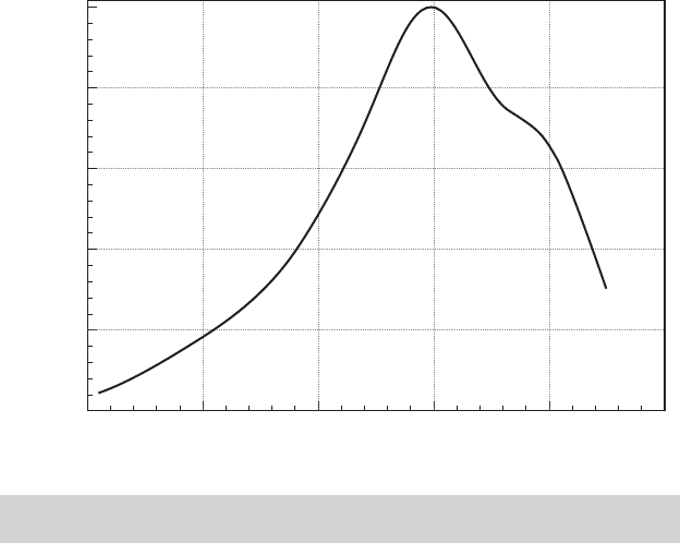
time were scaled as before. Figure 18.1 displays a kernel estimator of the estimates

of WTP

by this method. Note that the distribution is roughly centered on our earlier

estimate of $49.53. The density estimator reveals the heterogeneity in the population

of this parameter.

Willingness to pay measures computed as suggested above are ultimately based

on a ratio of two asymptotically normally distributed parameter estimators. In general,

ratios of normally distributed random variables do not have a ﬁnite variance. This often

becomes apparent when using the delta method, as it seems previously. A number of

writers, notably, Daly, Hess, and Train (2009), have documented the problem of extreme

CHAPTER 18

✦

Discrete Choices and Event Counts

781

25

0.0000

025 7550 100

0.0035

0.0069

0.0104

Density

0.0139

0.0174

WTP

Kernel Density Estimate for WTP

FIGURE 18.1

Estimated Willingness to Pay for Decreased Terminal

Time.

results of WTP computations, and why they should be expected. One solution suggested,

for example, by Train and Weeks (2005), Sonnier, Ainsle, and Otter (2007), and Scarpa,

Thiene, and Train (2008), is to recast the original model in willingness to pay space.In

the multinomial logit case, this amounts to a trivial reparameterization of the model.

Using our application as an example, we would write

= α

+ β

[GC

+ β

(

TTME

/β

TTME

] + γ

AIR

HINC

+ ε

= α

+ β

[GC

+ λ

(

TTME

] + γ

AIR

HINC

+ ε

This obviously returns the original model, though in the process, it transforms a linear

estimation problem into a nonlinear one. But, in principle, with the model reparame-

terized in “WTP space,” we have sidestepped the problem noted earlier – λ

(

TTME

is the

estimator of WTP with no further transformation of the parameters needed. As noted,

this will return the numerically identical results for a multinomial logit model. It will not

return the identical results for a mixed logit model, in which we write λ

TTME,i

= λ

(

TTME

+ θ

(

TTME

(

TTME,i

. Greene and Hensher (2010b) apply this method to the generalized

mixed logit model in Section 18.2.8.

18.2.11 PANEL DATA AND STATED CHOICE EXPERIMENTS

Panel data in the unordered discrete choice setting typically come in the form of se-

quential choices. Train (2009, Chapter 6) reports an analysis of the site choices of 258

anglers who chose among 59 possible ﬁshing sites for a total of 962 visits. Allenby and

Rossi (1999) modeled brand choice for a sample of shoppers who made multiple store

trips. The mixed logit model is a framework that allows the counterpart to a random

782

PART IV

✦

Cross Sections, Panel Data, and Microeconometrics

effects model. The random utility model would appear

ij,t

= x



ij,t

+ ε

ij,t

where conditioned on β

, a multinomial logit model applies. The random coefﬁcients

carry the common effects across choice situations. For example, if the random coefﬁ-

cients include choice-speciﬁc constant terms, then the random utility model becomes

essentially a random effects model. A modiﬁcation of the model that resembles Mund-

lak’s correction for the random effects model is

= β

+ z

+ u

where, typically, z

would contain demographic and socioeconomic information.

The stated choice experiment is similar to the repeated choice situation, with a

crucial difference. In a stated choice survey, the respondent is asked about his or her

preferences over a series of hypothetical choices, often including one or more that are

actually available and others that might not be available (yet). Hensher, Rose, and

Greene (2006) describe a survey of Australian commuters who were asked about hypo-

thetical commutation modes in a choice set that included the one they currently took

and a variety of proposed alternatives. Revelt and Train (2000) analyzed a stated choice

experiment in which California electricity consumers were asked to choose among al-

ternative hypothetical energy suppliers. The advantage of the stated choice experiment

is that it allows the analyst to study choice situations over a range of variation of the

attributes or a range of choices that might not exist within the observed, actual out-

comes. Thus, the original work on the MNL by McFadden et al. concerned survey data

on whether commuters would ride a (then-hypothetical) underground train system to

work in the San Francisco Bay area. The disadvantage of stated choice data is that

they are hypothetical. Particularly when they are mixed with revealed preference data,

the researcher must assume that the same preference patterns govern both types of

outcomes. This is likely to be a dubious assumption. One method of accommodating

the mixture of underlying preferences is to build different scaling parameters into the

model for the stated and revealed preference components of the model. Greene and

Hensher (2007) suggested a nested logit model that groups the hypothetical choices in

one branch of a tree and the observed choices in another.

18.2.12 AGGREGATE MARKET SHARE DATA—THE BLP RANDOM

PARAMETERS MODEL

We note, ﬁnally, an important application of the mixed logit model, the structural de-

mand model of Berry, Levinsohn, and Pakes (1995). (Demand models for differenti-

ated products such as automobiles [BLP (1995), Goldberg (1995)], ready-to-eat cereals

[Nevo (2001)], and consumer electronics [Das, Olley, and Pakes (1996)], have been

constructed using the mixed logit model with market share data.

A basic structure is

deﬁned for

Markets, denoted t = 1,...,T,

Consumers in the markets, denoted i = 1,...,n

Products, denoted j = 1,..., J.

We draw heavily on Nevo (2000) for this discussion.

CHAPTER 18

✦

Discrete Choices and Event Counts

783

The deﬁnition of a market varies by application; BLP analyzed the U.S. national auto-

mobile market for 20 years; Nevo examined a cross section of cities over 20 quarters so

the city-quarter is a market; Das et al. deﬁned a market as the annual sales to consumers

in particular income levels.

For market t, we base the analysis on average prices, p

, aggregate quantities q

consumer incomes y

observed product attributes, x

and unobserved (by the analyst)

product attributes, 

. The indirect utility function for consumer i, for product j in

market t is

ijt

= α

− p

) + x



+ 

+ ε

ijt

, (18-14)

where α

is the marginal utility of income and β

are marginal utilities attached to

speciﬁc observable attributes of the products. The fact that some unobservable product

attributes, 

will be reﬂected in the prices implies that prices will be endogenous

in a demand model that is based on only the observable attributes. Heterogeneity in

preferences is reﬂected (as we did earlier) in the formulation of the random parameters,



















γ w

v



, (18-15)

where d

is a vector of demographics such as gender and age while α, β, π, , γ , and 

are structural parameters to be estimated (assuming they are identiﬁed). A utility func-

tion is also deﬁned for an “outside good” that is (presumably) chosen if the consumer

chooses none of the brands, 1, . . . , J :

i0t

= α

+ 

+ π



+ ε

i0t

Since there is no variation in income across the choices, α

will fall out of the logit

probabilities, as we saw earlier. A normalization is used instead, u

i0t

= ε

i0t

, so that

comparisons of utilities are against the outside good. The resulting model can be recon-

structed by inserting (18-15) into (18-14),

ijt

= α

+ δ

, p

,

: α, β) + τ

ijt

, p

, v

, w

: π, ,γ,) + ε

ijt

= x



β − αp

+ 

= [−p

, x



]











γ w

v



The preceding model deﬁnes the random utility model for consumer i in market t. Each

consumer is assumed to purchase the one good that maximizes utility. The market share

of the j th product in this market is obtained by summing over the choices made by those

consumers. With the assumption of homogeneous tastes ( = 0 and γ = 0) and i.i.d.,

type I extreme value distributions for ε

ijt

, it follows that the market share of product

j is

exp(x



β − αp

+ 

)

1 +



k=1

exp(x



β − αp

+ 

)

The IIA assumptions produce the familiar problems of peculiar and unrealistic sub-

stitution patterns among the goods. Alternatives considered include a nested logit, a

“generalized extreme value” model and, ﬁnally, the mixed logit model, now applied to

the aggregate data.

784

PART IV

✦

Cross Sections, Panel Data, and Microeconometrics

Estimation cannot proceed along the lines of Section 18.2.7 because 

is unob-

served and p

is, therefore, endogenous. BLP propose, instead to use a GMM estimator,

based on the moment equations

E{[S

− s

, p

|α, β)]z

}=0

for a suitable set of instruments. Layering in the random parameters speciﬁcation, we

obtain an estimation based on method of simulated moments, rather than a maximum

simulated log likelihood. The simulated moments would be based on

w,v

, p

|α

, β

)] =

w,v



, p

|α

(w), β

(v)]



dF(w) dF(v).

These would be simulated using the method of Section 18.2.7.

18.3 RANDOM UTILITY MODELS FOR ORDERED

CHOICES

The analysts at bond rating agencies such as Moody’s and Standard and Poor provide an

evaluation of the quality of a bond that is, in practice, a discrete listing of the continuously

varying underlying features of the security. The rating scales are as follows:

Rating S&P Rating Moody’s Rating

Highest quality AAA Aaa

High quality AA Aa

Upper medium quality A A

Medium grade BBB Baa

Somewhat speculative BB Ba

Low grade, speculative B B

Low grade, default possible CCC Caa

Low grade, partial recovery possible CC Ca

Default, recovery unlikely C C

For another example, Netﬂix (http://www.netﬂix.com) is an Internet company that rents

movies. Subscribers order the ﬁlm online for download or home delivery of a DVD.

The next time the customer logs onto the Web site, they are invited to rate the movie

on a ﬁve-point scale, where ﬁve is the highest, most favorable rating. The ratings of

the many thousands of subscribers who rented that movie are averaged to provide a

recommendation to prospective viewers. As of April 5, 2009, the average rating of the

2007 movie National Treasure: Book of Secrets given by approximately 12,900 visitors

to the site was 3.8. Many other Internet sellers of products and services, such as Barnes

and Noble, Amazon, Hewlett Packard, and Best Buy, employ rating schemes such as

this. Many recently developed national survey data sets, such as the British Household

Panel Data Set (BHPS) (http://www.iser.essex.ac.uk/survey/bhps) and the German So-

cioeconomic Panel (GSOEP) (http://www.diw.de/en/soep), contain questions that elicit

self-assessed ratings of health, health satisfaction, or overall well-being. Like the other

examples listed, these survey questions are answered on a discrete scale, such as the

CHAPTER 18

✦

Discrete Choices and Event Counts

785

zero to 10 scale of the question about health satisfaction in the GSOEP. Ratings such as

these provide applications of the models and methods that interest us in this section.

For any individual respondent, we hypothesize that there is a continuously varying

strength of preferences that underlies the rating they submit. For convenience and

consistency with what follows, we will label that strength of preference “utility,” U

∗

Continuing the Netﬂix example, we describe utility as ranging over the entire real line:

−∞ < U

∗

< +∞

where i indicates the individual and m indicates the movie. Individuals are invited to

“rate” the movie on an integer scale from 1 to 5. Logically, then, the translation from

underlying utility to a rating could be viewed as a censoring of the underlying utility,

= 1if −∞< U

∗

≤ μ

= 2ifμ

< U

∗

≤ μ

= 3ifμ

< U

∗

≤ μ

= 4ifμ

< U

∗

≤ μ

= 5ifμ

< U

∗

< ∞.

The same mapping would characterize the bond ratings, since the qualities of bonds that

produce the ratings will vary continuously, and the self-assessed health and well-being

questions in the panel survey data sets based on an underlying utility or preference

structure. The crucial feature of the description thus far is that underlying the discrete

response is a continuous range of preferences. Therefore, the observed rating represents

a censored version of the true underlying preferences. Providing a rating of ﬁve could

be an outcome ranging from general enjoyment to wild enthusiasm. Note that the

thresholds, μ

, number (J − 1) where J is the number of possible ratings (here, ﬁve) –

J −1 values are needed to divide the range of utility into J cells. The thresholds are an

important element of the model; they divide the range of utility into cells that are then

identiﬁed with the observed outcomes. Importantly, the difference between two levels

of a rating scale (for example, one compared to two, two compared to three) is not the

same as on a utility scale. Hence we have a strictly nonlinear transformation captured

by the thresholds, which are estimable parameters in an ordered choice model.

The model as suggested thus far provides a crude description of the mechanism

underlying an observed rating. Any individual brings their own set of characteristics to

the utility function, such as age, income, education, gender, where they live, family situ-

ation, and so on, which we denote x

, x

,...,x

iK.

They also bring their own aggregate

of unmeasured and unmeasurable (by the statistician) idiosyncrasies, denoted ε

How

these features enter the utility function is uncertain, but it is conventional to use a linear

function, which produces a familiar random utility function,

∗

= β

+ β

+···+β

+ ε

Greene and Hensher (2010) provide a survey of ordered choice modeling. Other textbook and monograph

treatments include DeMaris (2004), Long (1997), Johnson and Abbot (1999), and Long and Freese (2006).

Introductions to the model also appear in journal articles such as Winship and Mare (1984), Becker and

Kennedy (1992), Daykin and Moffatt (2002), and Boes and Winkelmann (2006).

786

PART IV

✦

Cross Sections, Panel Data, and Microeconometrics

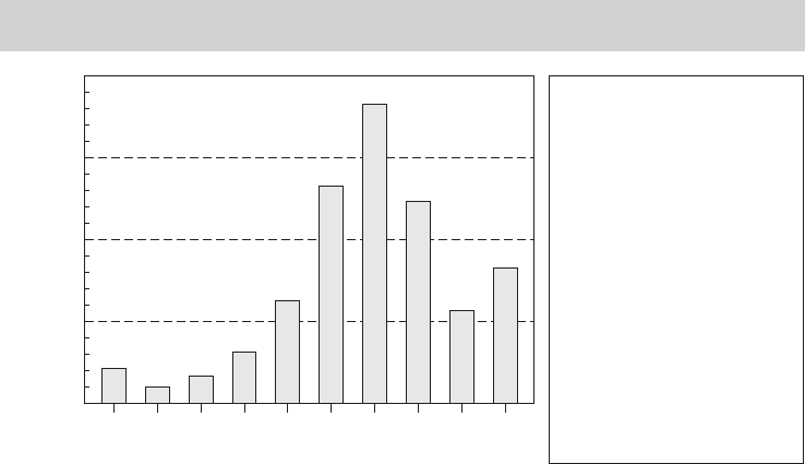
Example 18.2 Movie Ratings

The Web site http://www.IMDb.com invites visitors to rate movies that they have seen, in the

same fashion as the Netﬂix site. This site uses a 10 point scale. On December 1, 2008, they

reported the results in Figure 18.2 for the movie National Treasure: Book of Secrets for 41,771

users of the site. The ﬁgure at the left shows the overall ratings. The panel at the right shows

how the average rating varies across age, gender, and whether the rater is a U.S. viewer or not.

The rating mechanism we have constructed is

= 1if−∞ < x



β + ε

≤ μ

= 2ifμ

< x



β + ε

≤ μ

···

= 9ifμ

< x



β + ε

≤ μ

= 10 if μ

< x



β + ε

< ∞.

Relying on a central limit to aggregate the innumerable small inﬂuences that add up to the

individual idiosyncrasies and movie attraction, we assume that the random component, ε

is normally distributed with zero mean and (for now) constant variance. The assumption of

normality will allow us to attach probabilities to the ratings. In particular, arguably the most

interesting one is

Prob( R

= 10 |x

) = Prob[ε

>μ

− x



β].

The structure provides the framework for an econometric model of how individuals rate

movies (that they rent from Netﬂix). The resemblance of this model to familiar models of

binary choice is more than superﬁcial. For example, one might translate this econometric

model directly into a probit model by focusing on the variable

= 1ifR

= 10

= 0ifR

< 10.

Thus, the model is an extension of a binary choice model to a setting of more than two choices.

But, the crucial feature of the model is the ordered nature of the observed outcomes and the

correspondingly ordered nature of the underlying preference scale.

FIGURE 18.2

IMDb.com Ratings (http://www.imdb.com/title/

tt0465234/ratings).

Frequency

IMDb Vote

2,925

5,850

8,775

11,700

23456789101

Males

Females

Aged under 18

Males under 18

Females under 18

Aged 18–29

Males Aged 18–29

Females Aged 18–29

Aged 30–44

Males Aged 30–44

Females Aged 30–44

Aged 45+

Males Aged 45+

Females Aged 45+

US Users

Non-US Users

Votes

33,644

5,464

2,492

1,795

695

26,045

22,603

3,372

8,210

7,216

936

2,258

1,814

420

14,792

24,283

CHAPTER 18

✦

Discrete Choices and Event Counts

787

The model described here is an ordered choice model. (The choice of the normal

distribution for the random term makes it an ordered probit model.) Ordered choice

models are appropriate for a wide variety of settings in the social and biological sci-

ences. The essential ingredient is the mapping from an underlying, naturally ordered

preference scale to a discrete ordered observed outcome, such as the rating scheme just

described. The model of ordered choice pioneered by Aitcheson and Silvey (1957),

Snell (1964), and Walker and Duncan (1967) and articulated in its modern form by

Zavoina and McElvey (1975) has become a widely used tool in many ﬁelds. The num-

ber of applications in the current literature is large and increasing rapidly, including

•

Bond ratings [Terza (1985a)],

•

Congressional voting on a Medicare bill [McElvey and Zavoina (1975)],

•

Credit ratings [Cheung (1996) , Metz, and Cantor (2006)],

•

Driver injury severity in car accidents [Eluru, Bhat, and Hensher (2008)],

•

Drug reactions [Fu, Gordon, Liu, Dale, and Christensen (2004)],

•

Education [Machin and Vignoles (2005), Carneiro, Hansen, and Heckman (2003),

Cunha, Heckman, and Navarro (2007)],

•

Financial failure of ﬁrms [Hensher and Jones (2007)],

•

Happiness [Winkelmann (2005), Zigante (2007)],

•

Health status [Jones, Koolman, and Rice (2003)],

•

Life satisfaction [Clark, Georgellis, and Sanfey (2001), Groot and ven den Brink

(2003)],

•

Monetary policy [Eichengreen, Watson, and Grossman (1985)],

•

Nursing labor supply [Brewer, Kovner, Greene, and Cheng (2008)],

•

Obesity [Greene, Harris, Hollingsworth, and Maitra (2008)],

•

Political efﬁcacy [King, Murray, Salomon, and Tandon (2004)],

•

Pollution [Wang and Kockelman (2009)],

•

Promotion and rank in nursing [Pudney and Shields (2000)],

•

Stock price movements [Tsay (2005)],

•

Tobacco use [Harris and Zhao (2007), Kasteridis, Munkin, and Yen (2008)],

•

Work disability [Kapteyn et al. (2007)].

18.3.1 THE ORDERED PROBIT MODEL

The ordered probit model is built around a latent regression in the same manner as the

binomial probit model. We begin with

∗

= x



β + ε.

As usual, y

∗

is unobserved. What we do observe is

y = 0ify

∗

≤ 0

= 1if0< y

∗

≤ μ

= 2ifμ

< y

∗

≤ μ

= J if μ

J −1

≤ y

∗

which is a form of censoring. The μ’s are unknown parameters to be estimated with β.

788

PART IV

✦

Cross Sections, Panel Data, and Microeconometrics

0.1

f(⑀)

␤ⴕx

␮

␤ⴕx ␮

␤ⴕx

⑀

␮

␤ⴕx

y  0 y  1 y  2 y  3 y  4

0.2

0.3

0.4

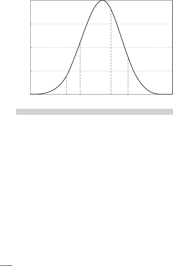
FIGURE 18.3

Probabilities in the Ordered Probit Model.

We assume that ε is normally distributed across observations.

For the same rea-

sons as in the binomial probit model (which is the special case of J = 1), we nor-

malize the mean and variance of ε to zero and one. We then have the following

probabilities:

Prob(y = 0 |x) = (−x



β),

Prob(y = 1 |x) = (μ

− x



β) − (−x



β),

Prob(y = 2 |x) = (μ

− x



β) − (μ

− x



β),

Prob(y = J |x) = 1 − (μ

J −1

− x



β).

For all the probabilities to be positive, we must have

0 <μ

<μ

< ···<μ

J −1

Figure 18.3 shows the implications of the structure. This is an extension of the uni-

variate probit model we examined in Chapter 17. The log-likelihood function and its

derivatives can be obtained readily, and optimization can be done by the usual means.

As usual, the partial effects of the regressors x on the probabilities are not equal

to the coefﬁcients. It is helpful to consider a simple example. Suppose there are three

categories. The model thus has only one unknown threshold parameter. The three

Other distributions, particularly the logistic, could be used just as easily. We assume the normal purely for

convenience. The logistic and normal distributions generally give similar results in practice.