Greene W.H. Econometric Analysis

Подождите немного. Документ загружается.

CHAPTER 18

✦

Discrete Choices and Event Counts

809

The conditional mean function for the three cases considered is

E[y

] = exp(x



β) = λ

The parameter P is picking up the scaling. A general result is that for all three variants

of the model,

Var[y

] = λ



1 + αλ

P−1



, where α = 1/θ.

Thus, the NB2 form has a variance function that is quadratic in the mean while the NB1

form’s variance is a simple multiple of the mean. There have been many other functional

forms proposed for count data models, including the generalized Poisson, gamma, and

Polya-Aeppli forms described in Winkelmann (2003) and Greene (2007a, Chapter 24).

The heteroscedasticity in the count models is induced by the relationship between

the variance and the mean. The single parameter θ picks up an implicit overall scaling, so

it does not contribute to this aspect of the model. As in the linear model, microeconomic

data are likely to induce heterogeneity in both the mean and variance of the response

variable. A speciﬁcation that allows independent variation of both will be of some virtue.

The result

Var[y

] = λ



1 + (1/θ)λ

P−1



suggests that a convenient platform for separately modeling heteroscedasticity will be

the dispersion parameter, θ, which we now parameterize as

= θ exp(z



δ).

Operationally, this is a relatively minor extension of the model. But, it is likely to

introduce quite a substantial increase in the ﬂexibility of the speciﬁcation. Indeed, a

heterogeneous Negbin P model is likely to be sufﬁciently parameterized to accommo-

date the behavior of most data sets. (Of course, the specialized models discussed in

Section 18.4.8, for example, the zero inﬂation models, may yet be more appropriate for

a given situation.)

Example 18.7 Count Data Models for Doctor Visits

The study by Riphahn et al. (2003) that provided the data we have used in numerous earlier

examples analyzed the two count variables DocVis (visits to the doctor) and HospVis (visits

to the hospital). The authors were interested in the joint determination of these two count

variables. One of the issues considered in the study was whether the data contained evidence

of moral hazard, that is, whether health care utilization as measured by these two outcomes

was inﬂuenced by the subscription to health insurance. The data contain indicators of two

levels of insurance coverage, PUBLIC, which is the main source of insurance, and ADDON,

which is a secondary optional insurance. In the sample of 27,326 observations (family/years),

24,203 individuals held the public insurance. (There is quite a lot of within group variation in

this. Individuals did not routinely obtain the insurance for all periods.) Of these 24,203, 23,689

had only public insurance and 514 had both types. (One could not have only the ADDON

insurance.) To explore the issue, we have analyzed the DocVis variable with the count data

models described in this section. The exogenous variables in our model are

= (1,Age, Education, Income, Kids, Public).

(Variables are described in Appendix Table F7.1.)

Table 18.14 presents the estimates of the several count models. In all speciﬁcations, the

coefﬁcient on PUBLIC is positive, large, and highly statistically signiﬁcant, which is consistent

with the results in the authors’ study. The various test statistics strongly reject the hypothesis

810

PART IV

✦

Cross Sections, Panel Data, and Microeconometrics

TABLE 18.14

Estimated Models for DOCVIS (standard errors in parentheses)

Negbin 2

Variable Poisson Negbin 2 Heterogeneous Negbin 1 Negbin P

Constant 0.7162 0.7628 0.7928 0.6848 0.6517

(0.03287) (0.07247) (0.07459) (0.06807) (0.07759)

Age 0.01844 0.01803 0.01704 0.01585 0.01907

(0.0003316) (0.0007915) (0.0008146) (0.0007042) (0.0008078)

Education −0.03429 −0.03839 −0.03581 −0.02381 −0.03388

(0.001797) (0.003965) (0.004036) (0.003702) (0.004308)

Income −0.4751 −0.4206 −0.4108 −0.1892 −0.3337

(0.02198) (0.04700) (0.04752) (0.04452) (0.05161)

Kids −0.1582 −0.1513 −0.1568 −0.1342 −0.1622

(0.007956) (0.01738) (0.01773) (0.01647) (0.01856)

Public 0.2364 0.2324 0.2411 0.1616 0.2195

(0.01328) (0.02900) (0.03006) (0.02678) (0.03155)

P 0.0000 2.0000 2.0000 1.0000 1.5473

(0.0000) (0.0000) (0.0000) (0.0000) (0.03444)

θ 0.0000 1.9242 2.6060 6.1865 3.2470

(0.0000) (0.02008) (0.05954) (0.06861) (0.1346)

δ (Female) 0.0000 0.0000 −0.3838 0.0000 0.0000

(0.0000) (0.0000) (0.02046) (0.0000) (0.0000)

δ (Married) 0.0000 0.0000 −0.1359 0.0000 0.0000

(0.0000) (0.0000) (0.02307) (0.0000) (0.0000)

ln L −104,440.3 −60,265.49 −60,121.77 −60,260.68 −60,197.15

of equidispersion. Cameron and Trivedi’s (1990) semiparametric tests from the Poisson model

(see Section 18.4.3 have t statistics of 22.147 for g

= μ

and 22.504 for g

= μ

. Both of

these are far larger than the critical value of 1.96. The LM statistic is 972,714.48, which is

also larger than the (any) critical value. On these bases, we would reject the hypothesis of

equidispersion. The Wald and likelihood ratio tests based on the negative binomial models

produce the same conclusion. For comparing the different negative binomial models, note

that Negbin 2 is the worst of the three by the likelihood function, although NB1 and NB2

are not directly comparable. On the other hand, note that in the NBP model, the estimate

of P is more than 10 standard errors from 1.0000 or 2.000, so both NB1 and NB2 are

rejected in favor of the unrestricted NBP form of the model. The NBP and the heterogeneous

NB2 model are not nested either, but comparing the log-likelihoods, it does appear that the

heterogeneous model is substantially superior. We computed the Vuong statistic based on

the individual contributions to the log-likelihoods, with v

= ln L

(NBP) − ln L

(NB2-H) . (See

Section 14.6.6). The value of the statistic is −3.27. On this basis, we would reject NBP in

favor of NB2-H. Finally, with regard to the original question, the coefﬁcient on PUBLIC is

larger than 10 times the estimated standard error in every speciﬁcation. We would conclude

that the results are consistent with the proposition that there is evidence of moral hazard.

18.4.6 TRUNCATION AND CENSORING IN MODELS FOR COUNTS

Truncation and censoring are relatively common in applications of models for counts.

Truncation arises as a consequence of discarding what appear to be unusable data,

such as the zero values in survey data on the number of uses of recreation facilities

[Shaw (1988), Bockstael et al. (1990)]. In this setting, a more common case which also

gives rise to truncation is on-site sampling. When one is interested in visitation by the

entire population, which will naturally include zero visits, but one draws their sample

CHAPTER 18

✦

Discrete Choices and Event Counts

811

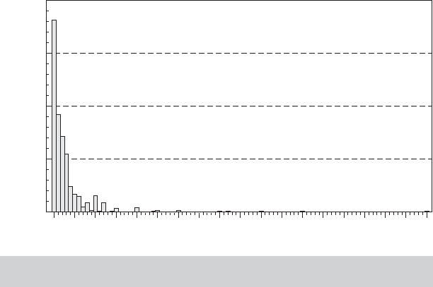
Frequency

Visits

436

872

1,308

1,744

10 15 20 25 30 35 40 45 50 55 60 65 70 75 80 85 9005

FIGURE 18.6

Number of Doctor Visits. 1988 Wave of GSOEP

Data.

“on-site,” the distribution of visits is truncated at zero by construction. Every visitor has

visited at least once. Shaw (1988), Englin and Shonkwiler (1995), Grogger and Carson

(1991), Creel and Loomis (1990), Egan and Herriges (2006), and Martinez-Espinera

and Amoako-Tuffour (2008) are among a number of studies that have treated trunca-

tion due to on-site sampling in environmental and recreation applications. Truncation

will also arise when data are trimmed to remove what appear to be unusual values.

Figure 18.6 displays a histogram for the number of doctor visits in the 1988 wave of the

GSOEP data that we have used in several examples. There is a suspiciously large spike

at zero and an extremely long right tail of what might seem to be atypical observations.

For modeling purposes, it might be tempting to remove these “non-Poisson” appearing

observations in these tails. (Other models might be a better solution.) The distribution

that characterizes what remains in the sample is a truncated distribution. Truncation is

not innocent. If the entire population is of interest, then conventional statistical infer-

ence (such as estimation) on the truncated sample produces a systematic bias known

as (of course) “truncation bias.” This would arise, for example, if an ordinary Poisson

model intended to characterize the full population is ﬁt to the sample from a truncated

population.

Censoring, in contrast, is generally a feature of the sampling design. In the applica-

tion in Example 18.9, the dependent variable is the self-reported number of extramarital

affairs in a survey taken by the magazine Psychology Today. The possible answers are

0, 1, 2, 3, 4–10 (coded as 7) and “monthly, weekly or daily” coded as 12. The two upper

categories are censored. Similarly, in the doctor visits data in the previous paragraph,

recognizing the possibility of truncation bias due to data trimming, we might, instead,

simply censor the distribution of values at 15. The resulting variable would take values

0, . . . , 14, “15 or more.” In both cases, applying conventional estimation methods leads to

predictable biases. However, it is also possible to reconstruct the estimators speciﬁcally

to account for the truncation or censoring in the data.

812

PART IV

✦

Cross Sections, Panel Data, and Microeconometrics

Truncation and censoring produce similar effects on the distribution of the random

variable and on the features of the population such as the mean. For the truncation

case, suppose that the original random variable has a Poisson distribution—all these

results can be directly extended to the negative binomial or any of the other models

considered earlier—with

P(y

= j |x

) = exp(−λ

)λ

/j! = P

i, j

If the distribution is truncated at value C—that is, only values C +1, . . . are observed—

then the resulting random variable has probability distribution

P(y

= j |x

, y

> C) =

P(y

= j |x

)

P(y

> C |x

)

P(y

= j |x

)

1 − P(y

≤ C |x

)

The original distribution must be scaled up so that it sums to one for the cells that

remain in the truncated distribution. The leading case is truncation at zero, that is, “left

truncation,” which, for the Poisson model produces

P(y

= j |x

, y

> 0) =

exp(−λ

)λ

j![1 − exp(−λ

)]

i, j

1 − P

i,0

, j = 1,....

[See, e.g., Mullahy (1986), Shaw (1988), Grogger and Carson (1991), Greene (1998),

and Winkelmann (1987).] The conditional mean function is

E(y

, y

> 0) =

[1 − exp(−λ

)]

∞



j=1

j exp(−λ

)λ

[1 − exp(−λ

)]

>λ

The second equality results because the sum can be started at zero—the ﬁrst term

is zero—and this produces the expected value of the original variable. As might be

expected, truncation “from below” has the effect of increasing the expected value. It

can be shown that it decreases the conditional variance however. The partial effects are

∂ E[y

, y

> 0]

∂x



1 − P

i,0

− λ

i,0



1 − P

i,0





β. (18-23)

The term outside the brackets is the partial effects in the absence of the truncation while

the bracketed term rises from slighter greater than 0.5 to 1.0 as λ

increases from just

above zero.

Example 18.8 Major Derogatory Reports

In Section 17.5.6 and Examples 17.9 and 17.22, we examined a binary choice model for the

accept/reject decision for a sample of applicants for a major credit card. Among the variables

in that model is “Major Derogatory Reports” (MDRs). This is an interesting behavioral variable

in its own right that can be appropriately modeled using the count data speciﬁcations in this

chapter. In the sample of 13,444 individuals, 10,833 had zero MDRs while the values for the

remaining 2,561 ranged from 1 to 22. This preponderance of zeros exceeds by far what one

would anticipate in a Poisson model that was dispersed enough to produce the distribution

of remaining individuals. As we will pursue an Example 18.11, a natural approach for these

data is to treat the extremely large block of zeros explicitly in an extended model. For present

purposes, we will consider the nonzero observations apart from the zeros and examine the

effect of accounting for left truncation at zero on the estimated models. Estimation results

are shown in Table 18.15. The ﬁrst column of results compared to the second shows the

CHAPTER 18

✦

Discrete Choices and Event Counts

813

TABLE 18.15

Estimated Truncated Poison Regression Model (

ratios in

parentheses)

Poisson Full Sample Poisson Truncated Poisson

Constant 0.8756 (17.10) 0.8698 (16.78) 0.7400 (11.99)

Age 0.0036 (2.38) 0.0035 (2.32) 0.0049 (2.75)

Income −0.0039 (−4.78) −0.0036 (−3.83) −0.0051 (−4.51)

OwnRent −0.1005 (−3.52) −0.1020 (−3.56) −0.1415 (−4.18)

Self-Employed −0.0325 (−0.62) −0.0345 (−0.66) −0.0515 (−0.82)

Dependents 0.0445 (4.69) 0.0440 (4.62) 0.0606 (5.48)

MthsCurAdr 0.00004 (0.23) 0.00005 (0.25) 0.00007 (0.30)

ln L −5,379.30 −5,378.79 −5,097.08

Average Partial Effects

Age 0.0017 0.0085 0.0084

Income −0.0018 −0.0087 −0.0089

OwnRent −0.0465 −0.2477 −0.2460

Self-Employed −0.0150 −0.0837 −0.0895

Dependents 0.0206 0.1068 0.1054

MthsCurAdr 0.00002 0.00012 0.00013

Cond’l. Mean 0.4628 2.4295 2.4295

Scale factor 0.4628 2.4295 1.7381

suspected impact of incorrectly including the zero observations. The coefﬁcients change only

slightly, but the partial effects are far smaller when the zeros are included in the estimation.

It was not possible to ﬁt the truncated negative binomial with these data.

Censoring is handled similarly. The usual case is “right censoring,” in which realized

values greater than or equal to C are all given the value C. In this case, we have a two-

part distribution [see Terza (1985b)]. The observed random variable, y

is constructed

from an underlying random variable, y

∗

= Min(y

∗

, C).

Probabilities are constructed using the axioms of probability. This produces

Prob(y

= j |x

) = P

i, j

, j = 0, 1,...,C − 1,

Prob(y

= C |x

) =

∞



j=C

i, j

= 1 −

C−1



j=0

i, j

In this case, the conditional mean function is

E[y

] =

C−1



j=0

i, j

∞



j=C

i, j

∞



j=0

i, j

−

∞



j=C

( j − C)P

i, j

= λ

−

∞



j=C

( j − C)P

i, j

<λ

814

PART IV

✦

Cross Sections, Panel Data, and Microeconometrics

The inﬁnite sum is computed by using the complement. Thus,

E[y

] = λ

−

⎡

⎣

∞



j=0

( j − C)P

i, j

−

C−1



j=0

( j − C)P

i, j

⎤

⎦

= λ

−

(

− C

)

C−1



j=0

( j − C)P

i, j

= C −

C−1



j=0

(C − j)P

i, j

Example 18.9 Extramarital Affairs

In 1969, the popular magazine Psychology Today published a 101-question survey on sex

and asked its readers to mail in their answers. The results of the survey were discussed in

the July 1970 issue. From the approximately 2,000 replies that were collected in electronic

form (of about 20,000 received), Professor Ray Fair (1978) extracted a sample of 601 ob-

servations on men and women then currently married for the ﬁrst time and analyzed their

responses to a question about extramarital affairs. Fair’s analysis in this frequently cited study

suggests several interesting econometric questions. [In addition, his 1977 companion paper

in Econometrica on estimation of the tobit model contributed to the development of the EM

algorithm, which was published by and is usually associated with Dempster, Laird, and Rubin

(1977).]

Fair used the tobit model that we discuss in Chapter 19 as a platform The nonexperimental

nature of the data (which can be downloaded from the Internet at http://fairmodel.econ.yale

.edu/rayfair/work.ss.htm and are given in Appendix Table F18.1). provides a laboratory case

that we can use to examine the relationships among the tobit, truncated regression, and

probit models. Although the tobit model seems to be a natural choice for the model for these

data, given the cluster of zeros, the fact that the behavioral outcome variable is a count that

typically takes a small value suggests that the models for counts that we have examined in

this chapter might be yet a better choice. Finally, the preponderance of zeros in the data that

initially motivated the tobit model suggests that even the standard Poisson model, although

an improvement, might still be inadequate. We will pursue that aspect of the data later. In this

example, we will focus on just the censoring issue. Other features of the models and data

are reconsidered in the exercises.

The study was based on 601 observations on the following variables (full details on data

coding are given in the data ﬁle and Appendix Table F18.1):

y = number of affairs in the past year, 0, 1, 2, 3, 4–10 coded as 7

“monthly, weekly, or daily,” coded as 12. Sample mean = 1.46

Frequencies = (451, 34, 17, 19, 42, 38),

= sex = 0 for female, 1 for male. Sample mean = 0.476,

= age. Sample mean = 32.5,

= number of years married. Sample mean = 8.18,

= children, 0 = no, 1 = yes. Sample mean = 0.715,

= religiousness, 1 = anti, ...,5 = very. Sample mean = 3.12,

= education, years, 9 = grade school, 12 = high school, ...,20= Ph.D or other Sample

mean = 16.2,

= occupation, “Hollingshead scale,” 1–7. Sample mean = 4.19,

= self-rating of marriage, 1 = very unhappy, ...,5 = very happy. Sample mean = 3.93.

CHAPTER 18

✦

Discrete Choices and Event Counts

815

TABLE 18.16

Censored Poisson and Negative Binomial Distributions

Poisson Regression Negative Binomial Regression

Standard Marginal Standard Marginal

Variable Estimate Error Effect Estimate Error Effect

Based on Uncensored Poisson Distribution

Constant 2.53 0.197 — 2.19 0.859 —

−0.0322 0.00585 −0.0470 −0.0262 0.0180 −0.00393

0.116 0.00991 0.168 0.0848 0.0401 0.127

−0.354 0.0309 −0.515 −0.422 0.171 −0.632

0.0798 0.0194 0.116 0.0604 0.0909 0.0906

−0.409 0.0274 −0.596 −0.431 0.167 −0.646

α 7.015 0.945

ln L −1,427.037 −728.2441

Based on Poisson Distribution Right Censored at y = 4

Constant 1.90 0.283 — 4.79 1.16 —

−0.0328 0.00838 −0.0235 −0.0166 0.0250 −0.00428

0.105 0.0140 0.0755 0.174 0.0568 0.045

−0.323 0.0437 −0.232 −0.723 0.198 −0.186

0.0798 0.0275 0.0572 0.0900 0.116 0.0232

−0.390 0.0391 −0.279 −0.854 0.216 −0.220

α 9.40 1.35

ln L −747.7541 −482.0505

The tobit model was ﬁt to y using a constant term and all eight variables. A restricted model

was ﬁt by excluding z

, z

, and z

, none of which was individually statistically signiﬁcant in

the model. We are able to match exactly Fair’s results for both equations. The tobit model

should only be viewed as an approximation for these data. The dependent variable is a

count, not a continuous measurement. The Poisson regression model, or perhaps one of

the many variants of it, should be a preferable modeling framework. Table 18.16 presents

estimates of the Poisson and negative binomial regression models. There is ample evidence

of overdispersion in these data; the t ratio on the estimated overdispersion parameter is

7.015/0.945 = 7.42, which is strongly suggestive. The large absolute value of the coefﬁcient

is likewise suggestive.

Responses of 7 and 12 do not represent the actual counts. It is unclear what the effect

of the ﬁrst recoding would be, because it might well be the mean of the observations in this

group. But the second is clearly a censored observation. To remove both of these effects,

we have recoded both the values 7 and 12 as 4 and treated this observation (appropriately)

as a censored observation, with 4 denoting “4 or more.” As shown in the third and fourth

sets of results in Table 18.16, the effect of this treatment of the data is greatly to reduce

the measured effects. Although this step does remove a deﬁciency in the data, it does not

remove the overdispersion; at this point, the negative binomial model is still the preferred

speciﬁcation.

18.4.7 PANEL DATA MODELS

The familiar approaches to accommodating heterogeneity in panel data have fairly

straightforward extensions in the count data setting. [Hausman, Hall, and Griliches

(1984) give full details for these models.] We will examine them for the Poisson model.

The authors [and Allison (2000)] also give results for the negative binomial model.

816

PART IV

✦

Cross Sections, Panel Data, and Microeconometrics

18.4.7.a Robust Covariance Matrices for Pooled Estimators

The standard asymptotic covariance matrix estimator for the Poisson model is

Est. Asy. Var[

β] =



−

∂

ln L

∂

β∂





−1





i=1





−1

= [X



X]

−1

where

 is a diagonal matrix of predicted values. The BHHH estimator is

Est. Asy. Var[

β] =





i=1



∂ ln P

∂



∂ ln P

∂







−1





i=1



−









−1

= [X



−1

where

E is a diagonal matrix of residuals. The Poisson model is one in which the MLE is

robust to certain misspeciﬁcations of the model, such as the failure to incorporate latent

heterogeneity in the mean (that is, one ﬁts the Poisson model when the negative binomial

is appropriate). In this case, a robust covariance matrix is the “sandwich” estimator,

Robust Est. Asy. Var[

β] = [X



X]

−1



X][X



X]

−1

which is appropriate to accommodate this failure of the model. It has become common

to employ this estimator with all speciﬁcations, including the negative binomial. One

might question the virtue of this. Because the negative binomial model already accounts

for the latent heterogeneity, it is unclear what additional failure of the assumptions of

the model this estimator would be robust to. The questions raised in Section 14.8.3 and

14.8.4 about robust covariance matrices would be relevant here.

A related calculation is used when observations occur in groups that may be corre-

lated. This would include a random effects setting in a panel in which observations have

a common latent heterogeneity as well as more general, stratiﬁed, and clustered data

sets. The parameter estimator is unchanged in this case (and an assumption is made

that the estimator is still consistent), but an adjustment is made to the estimated asymp-

totic covariance matrix. The calculation is done as follows: Suppose the n observations

are assembled in G clusters of observations, in which the number of observations in

the i th cluster is n

. Thus,



i=1

= n. Denote by β the full set of model parameters

in whatever variant of the model is being estimated. Let the observation-speciﬁc gra-

dients and Hessians be g

= ∂ ln L

/∂β = (y

− λ

and H

= ∂

ln L

/∂β∂β



−λ



. The uncorrected estimator of the asymptotic covariance matrix based on the

Hessian is

=−H

−1

⎛

⎝

−



i=1



j=1

⎞

⎠

−1

The corrected asymptotic covariance matrix is

Est. Asy. Var[

β] = V



G − 1



⎡

⎣



i=1

⎛

⎝



j=1

⎞

⎠

⎛

⎝



j=1

⎞

⎠



⎤

⎦

CHAPTER 18

✦

Discrete Choices and Event Counts

817

Note that if there is exactly one observation per cluster, then this is G/(G − 1) times

the sandwich (robust) estimator.

18.4.7.b Fixed Effects

Consider ﬁrst a ﬁxed effects approach. The Poisson distribution is assumed to have

conditional mean

log λ

= β



+ α

, (18-24)

where now, x

has been redeﬁned to exclude the constant term. The approach used

in the linear model of transforming y

to group mean deviations does not remove the

heterogeneity, nor does it leave a Poisson distribution for the transformed variable.

However, the Poisson model with ﬁxed effects can be ﬁt using the methods described

for the probit model in Section 17.4.3. The extension to the Poisson model requires only

the minor modiﬁcations, g

=(y

−λ

) and h

=−λ

. Everything else in that deriva-

tion applies with only a simple change in the notation. The ﬁrst-order conditions for

maximizing the log-likelihood function for the Poisson model will include

∂ ln L

∂α



t=1

− e

) = 0 where μ

= e



This implies an explicit solution for α

in terms of β in this model,

ˆα

= ln



(1/T

)



t=1

(1/T

)



t=1

ˆμ



= ln



¯y

ˆμ



. (18-25)

Unlike the regression or the probit model, this does not require that there be within-

group variation in y

—all the values can be the same. It does require that at least one

observation for individual i be nonzero, however. The rest of the solution for the ﬁxed

effects estimator follows the same lines as that for the probit model. An alternative

approach, albeit with little practical gain, would be to concentrate the log-likelihood

function by inserting this solution for α

back into the original log-likelihood, and then

maximizing the resulting function of β. While logically this makes sense, the approach

suggested earlier for the probit model is simpler to implement.

An estimator that is not a function of the ﬁxed effects is found by obtaining the

joint distribution of (y

,...,y

) conditional on their sum. For the Poisson model, a

close cousin to the multinomial logit model discussed earlier is produced:



, y

,...,y



i=1







t=1





t=1



t=1

, (18-26)

where



β+α



t=1



β+α





t=1



. (18-27)

The contribution of group i to the conditional log-likelihood is

ln L



t=1

ln p

818

PART IV

✦

Cross Sections, Panel Data, and Microeconometrics

Note, once again, that the contribution to ln L of a group in which y

= 0 in every

period is zero. Cameron and Trivedi (1998) have shown that these two approaches give

identical results.

Hausman, Hall, and Griliches (1984) (HHG) report the following conditional den-

sity for the ﬁxed effects negative binomial (FENB) model:



, y

,...,y



t=1







1 +



t=1









t=1









t=1



t=1



t=1

(y

+ λ

)

(1 + y

)(λ

)

which is free of the ﬁxed effects. This is the default FENB formulation used in popular

software packages such as SAS, Stata, and LIMDEP. Researchers accustomed to the

admonishments that ﬁxed effects models cannot contain overall constants or time-

invariant covariates are sometimes surprised to ﬁnd (perhaps accidentally) that this

ﬁxed effects model allows both. [This issue is explored at length in Allison (2000) and

Allison and Waterman (2002).] The resolution of this apparent contradiction is that the

HHG FENB model is not obtained by shifting the conditional mean function by the

ﬁxed effect, ln λ

= x



β + α

, as it is in the Poisson model. Rather, the HHG model is

obtained by building the ﬁxed effect into the model as an individual speciﬁc θ

in the

Negbin 1 form in (18-22). The conditional mean functions in the models are as follows

(we have changed the notation slightly to conform to our earlier formulation):

NB1(HHG): E[y

] = θ

= θ

exp(x



β),

NB2: E[y

] = exp(α

)φ

= λ

= exp(x



β + α

The conditional variances are

NB1(HHG): Var[y

] = θ

[1 + θ

NB2: Var[y

] = λ

[1 + θλ

Letting μ

= ln θ

, it appears that the HHG formulation does provide a ﬁxed effect in

the mean, as now, E[y

] = exp(x



β + μ

). Indeed, by this construction, it appears

(as the authors suggest) that there are separate effects in both the mean and the variance.

They make this explicit by writing θ

= exp(μ

)γ

so that in their model,

E[y

] = γ

exp(x



β + μ

Var[y

] = γ

exp(x



β + μ

)/[1 + γ

exp(μ

)].

The contradiction arises because the authors assert that μ

and γ

are separate parame-

ters. In fact, they cannot vary separately only θ

can vary autonomously. The ﬁrm-speciﬁc

effect in the HHG model is still isolated in the scaling parameter, which falls out of the

conditional density. The mean is homogeneous, which explains why a separate constant,

or a time-invariant regressor (or another set of ﬁrm-speciﬁc effects) can reside there.

[See Greene (2007d) and Allison and Waterman (2002) for further discussion.]

18.4.7.c Random Effects

The ﬁxed effects approach has the same ﬂaws and virtues in this setting as in the

probit case. It is not necessary to assume that the heterogeneity is uncorrelated with