Griffiths D.F., Higham D.J. Numerical Methods for Ordinary Differential Equations: Initial Value Problems

Подождите немного. Документ загружается.

76 6. Linear Multistep Methods—III

Example 6.1

Use Euler’s method to solve the IVP (see Example 1.9)

(t) = −8x(t) − 40(3e

−t/8

− 1), x(0) = 100.

We know that the exact solution of this problem is given by

x(t) =

1675

−8t

320

−t/8

+ 5.

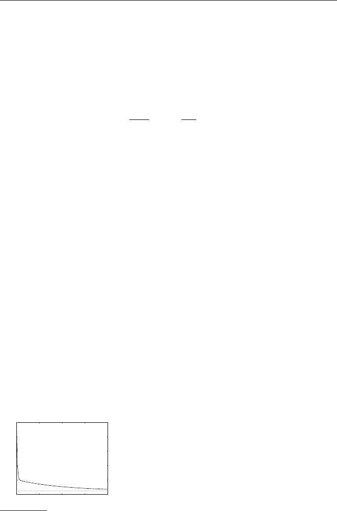
This function is shown in Figure 6.1. The temperature x(t) drops quite rapidly

from 100

◦

C to room temperature (about 20

◦

C) and then falls slowly to the

exterior temperature (about 5

◦

C).

Turning now to the numerical solution, Euler’s method applied to this ODE

gives

n+1

= (1 − 8h)x

+ h



120e

−t

+ 40



, n = 0, 1, 2, . . . ,

with t

= nh and x

= 100.

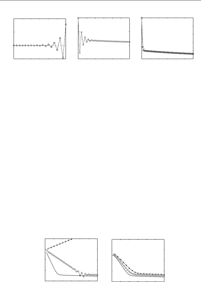
The leftmost graph in Figure 6.2 shows x

versus t

when h = 1/3. The nu-

merical solution has ever-increasing os cillations—a classic symptom of numeri-

cal instability—reaching a maximum amplitude of 10

. The numerical solution

bears no resemblance to the exact solution shown in Figure 6.1.

Reducing h (slightly) to 1/5 has a dramatic eﬀect on the solution (middle

graph): it now decays in time while continuing to oscillate until about t ≈ 2,

after which point it becomes a smooth curve.

When h is further reduced to 1/9 the solution rese mbles the exact solution,

but the solid and broken curves do not become close until t ≈ 0.5.

In Figure 6.3 we plot the GEs (GE) |x(nh) − x

| on a log-linear sc ale.

The linear growth of the GE on this scale for h = 1/3 suggests exponential

growth. In contrast, for h = 1/5, the error decays exponentially over the interval

0 4 8 12 16

100

u(t)

Fig. 6.1

The exact solution to Example 6.1

If the GE were to vary exponentially with n, e

= c r

, then log e

= n log r+log c

and a graph of log e

versus n would be a straight line with slope log r . When r > 1

the slope would be positive, corresponding to exponential growth, while the slope

would be negative if 0 < r < 1, corresponding to exponential decay.

6.1 Absolute Stability—Motivation 77

1 2 3 4 5 6

−5

x 10

1 2 3 4 5 6

−50

100

1 2 3 4 5 6

100

Fig. 6.2 Solutions to Example 6.1 using Euler’s method with h = 1/3 (left),

h = 1/5 (middle) and h = 1/9 (right). The exact solution of the IVP is shown

as a broken curve

0 ≤ t ≤ 4 where it reaches a level of about about 10

−3

. Were we to be interested

in an accuracy of about 1

◦

C, this would be achieved at around t = 1.8 h.

For h = 1/9 there is a more rapid initial exponential decay of the error until

it, too, levels out, at a similar value of about 10

−3

at t = 1.3 h.

The theory that we shall present below can be used to show (see Exam-

ple 6.7) that Euler’s method suﬀers a form of instability for this IVP when

h ≥ 1/4; this is clearly supported by the numerical evidence we have pre-

sented. This is typical: Euler’s me thod is of no practical use for problems with

exponentially decaying solutions unless h is small enough. Furthermore, when

h is chosen small enough to avoid exponential growth of the GE, the accuracy

of the long-term solution may be much higher than is required.

This behaviour is caused by the exponent e

−8t

in the complementary func-

tion; had it been e

−80t

we would have needed to take h to be 10 times smaller

and we would have generated, as a consequence, a numerical solution that was

10 times more accurate. Thus, in this problem, we are forced to choose a small

value of h in order to avoid instability and, while this will produce a solu-

1 2 3 4 5 6

−4

−2

1 2 3 4 5 6

−4

−2

Fig. 6.3 The GEs associated with the solutions to Example 6.1 using Euler’s

method (left) and the backward Euler method (right) with h = 1/3 (+), h =

1/5 (◦), and h = 1/9 (•)

78 6. Linear Multistep Methods—III

tion of high accuracy, it is likely to be more accurate than required by the

application—the method is ineﬃc ient since we have expended more eﬀort than

necessary when only moderate accuracy is called for.

We now contrast this behaviour with that of the backward Euler method:

n+1

= x

− 8hx

n+1

+ h



120e

−t

n+1

+ 40



, n = 0, 1, 2, . . . ,

which is rearranged to read

n+1

1 + 8h



+ h(120e

−t

n+1

+ 40)



, n = 0, 1, 2, . . . ,

with t

n+1

= (n + 1)h and x

= 100.

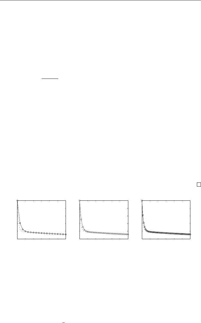
Solutions corresponding to h = 1/3, 1/5, 1/9 are shown in Figure 6.4. Com-

paring with Figure 6.2 it is evident that there are no oscillations and the nu-

merical solutions are reasonable approximations of the exact solution for each

of the values of h. The behaviour is such that small changes to h lead to small

changes in the numerical solutions (and associated GEs)—this is a desirable,

stable feature.

The local truncation errors for forward and backward Euler methods are

equal but opposite in sign. However, the way that these errors propagate is

clearly diﬀerent. In this example the backward Euler method is much superior

to that of the Euler method since we are able to choose h on grounds of accuracy

alone without having to be concerned with exponentially growing oscillations

for larger values of h.

1 2 3 4 5 6

100

1 2 3 4 5 6

100

1 2 3 4 5 6

100

Fig. 6.4 Solutions to Example 6.1 using the backward Euler method with

h = 1/3 (left), h = 1/5 (middle), and h = 1/9 (right). The exact solution of

the IVP is shown as a broken curve

Example 6.2

Use the forward and backward Euler methods to solve the IVP (see (1.16))

(t) = −

(x(t) − 5 − 5025e

−8t

), x(0) = 100.

6.2 Absolute Stability 79

Compare the results produced with those of the previous example which has

the same exact s olution (see Example 1.9).

The forward and backward Euler me thods are, respectively,

n+1

= (1 −

h)x

− h(5 − 5025e

−8t

n+1

1 + h/8



− h(5 − 5025e

−8t

n+1

)



with x

= 100 in each case. The GEs obtained when these methods are deployed

with h = 1/3 and 1/9 are shown in Figure 6.5. In both cases the GEs are

quite large over the interval of integration and decay slowly (proportional to

−t/8

). However, the most important feature in the present context is that

there is no indication of the exponential growth that we saw in the previous

example with Euler’s method with h = 1/3. In this example the forcing function

decays rapidly relative to the solutions of the homoge neous equation (e

−8t

versus e

−t/8

), whereas the roles are reversed in Example 6.1. This suggests

that the exponentially growing oscillations observed in Figure 6.2 with h = 1/3

are associated with rapidly decaying solutions of the homogeneous equation.

This is the motivation for studying homogeneous equations in the remainder

of this chapter.

6.2 Absolute Stability

The numerical results for Examples 6.1 and 6.2 lead us to absolute stability

theory, in which we examine the eﬀect of applying (convergent) LMMs to the

model scalar problem

(t) = λx(t), (6.1)

1 2 3 4 5 6

−4

−2

1 2 3 4 5 6

−4

−2

Fig. 6.5 The GEs associated with the solutions to Example 6.2 using Euler’s

method (left) and the backward Euler method (right) with h = 1/3 (+) and

h = 1/9 (•)

80 6. Linear Multistep Methods—III

in which λ may be complex

and has negative real part: <(λ) < 0. The general

solution has the form x(t) = c e

λt

in which c is an arbitrary constant. Hence,

x(t) → 0 as t → ∞, regardless of the value of c.

Our aim is to determine those LMMs which, when applied to (6.1), give

solutions {x

} that also tend to zero as t

→ ∞ with a given ﬁxed step size

h. Note that this property is diﬀerent from that used by convergence theory,

which also required the limit n → ∞, since h is now ﬁxed. This notion has

proved, perhaps surprisingly, to be both important and useful over many years

and we formalize our aspirations by the following deﬁnition.

Deﬁnition 6.3 (Absolute Stability)

An LMM is said to be absolutely stable if, when applied to the test problem

(t) = λx(t) with <(λ) < 0 and a given value of

h = hλ,

its solutions tend to

zero as n → ∞ for any choice of starting values.

Our deﬁnition of absolute stability is motivated by the idea of asking for

the numerical method to reproduce the long-term behaviour of the model ODE

(6.1). However, from Section 5.3 it should be clear that this condition is very

similar to the requirement that the GE should be damped as time increases—

this is the property that we looked at in Example 6.1. Hence, absolute stability

is an important factor in the control of the GE. Applying the general two-step

LMM (see Equation (4.13)) to the ODE x

(t) = λx(t) we have

n+2

+ α

n+1

+ α

= hλ(β

n+2

+ β

n+1

+ β

which can be rearranged to give the two-step linear diﬀerence equation

(1 −

hβ

n+2

+ (α

−

hβ

n+1

+ (α

−

hβ

= 0. (6.2)

This equation is relatively easy to analyse since it is a homogeneous linear

diﬀerence equation with constant coeﬃcients (see Appendix D). It has solutions

of the form x

= ar

, where r is a root of the auxiliary equation

(1 −

hβ

+ (α

−

hβ

)r + (α

−

hβ

) = 0. (6.3)

We denote the polynomial on the left-hand side by p(r). Notice that

p(r) = ρ(r) −

hσ(r).

The reason for allowing λ to be complex will become clear in Chapter 7 during

the application to systems of diﬀerential equations.

We introduce the single parameter

h since the parameters h and λ occur only as

the product hλ.

6.2 Absolute Stability 81

We refer to p(r) as the stability polynomial of the LMM; it is a polynomial of

degree 2 whose coeﬃcients depend (linearly) on the parameter

This stability p olynomial will have two roots, r

and r

, and so (6.2) will

have the general solution

= ar

+ br

for arbitrary constants a and b provided that r

6= r

order to have |x

| → 0

as n → ∞ for any choices of a and b, it is necessary to have |r

| < 1 and |r

| < 1,

i.e., the polynomial p(r) must satisfy the strict root condition (Deﬁnition 5.4).

This gives the following result.

Lemma 6.4

An LMM is absolutely stable for a given value of

h = λh if, and only if, its

stability polynomial p(r) satisﬁes the strict root condition (Deﬁnition 5.4).

An LMM will not, in general, be absolutely stable for every choice of

h, so we

are led to deﬁne the following.

Deﬁnition 6.5 (Region of Absolute Stability)

The set of values R in the complex

h-plane for which an LMM is absolutely

stable forms its region of absolute stability.

We must, therefore, address the question of whether, and for what values

h, the roots of p(r) satisfy |r| < 1. Cases where λ is real (and negative) are

easier to analyse so, for these, we deﬁne the following.

Deﬁnition 6.6 (Interval of Ab solute Stability)

The interval of absolute stability of an LMM is the largest interval of the form

= (

, 0), with

< 0, for which the LMM is absolutely stable for all real

values of

h ∈ R

The interval of absolute stability is found by looking at the intersection of

the region of absolute stability with the negative real

h axis.

The case of equality is unimportant since it could be countered by making a small

change to the value of h.

82 6. Linear Multistep Methods—III

Example 6.7

Find the region of absolute stability of Euler’s me thod: x

n+1

− x

= hf

Applied to x

(t) = λx(t) we have f

≡ f(t

, x

) = λx

so that

n+1

= x

+ hλx

= (1 +

h)x

This has stability polynomial p(r) = r − 1 −

h with the single root r

= 1 +

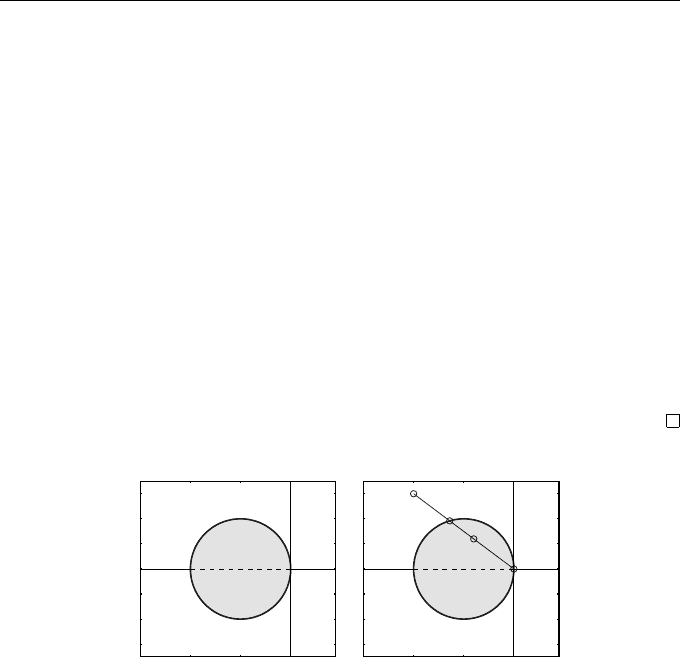
The region of absolute stability is, therefore, the open disc |1 +

h| < 1 whose

boundary is the circle of radius 1 centred at

h = −1. To see this, let

h = bx + iby,

then the boundary equation |1 +

= 1 leads to (bx + 1)

+ by

= 1.

h is real, the interval of absolute stability is given by

−1 < 1 +

h < 1,

which leads to

h ∈ (−2, 0). See Figure 6.6.

−3 −2 −1 0

−1.5

−1

−0.5

0.5

1.5

ℜ(

ℑ(

−3 −2 −1 0

−1.5

−1

−0.5

0.5

1.5

ℜ(

ℑ(

Fig. 6.6 The region of absolute stability for Euler’s method (shaded) and the

interval of absolute stability (broken line). On the right the line OA is the locus

of the points (−4h, 3h) for Example 6.8

If Euler’s method were to be applied to x

(t) = −8x(t), then

h = −8h and

absolute stability would require h < 1/4. Similarly, for x

= −80x, we would

have

h = −80h and absolute stability would require h < 1/40. This is the reason

that sensible results were computed with Euler’s method in Example 6.1 only

when h < 1/4.

Example 6.8

What is the largest value of h that can be used so that Euler’s method is

absolutely stable when used to solve the ODE x

(t) = λx(t) with λ = −3 + 4i?

6.2 Absolute Stability 83

In this case

h = h(−4 + 3i), |1 +

h| = |1 + h(−4 + 3i)|, and

|1 +

= |1 + h(−4 + 3i)|

= (1 − 4h)

+ 9h

Since |1 +

h| < 1 is equivalent to |1 +

− 1 < 0 we calculate

|1 +

− 1 = h(−8 + 25h)

and conclude that the right-hand side will be negative if h < 8/25.

To interpret the situation geometrically, let

h = bx + iby, where bx = −4h

and by = 3h. As h varies, the locus of the points (−4h, 3h) is a straight line in

the complex

h-plane having equation by = −

bx—this is shown as the line OA

in Figure 6.6 (right). The indicated points on this line are at h = 2/5, 8/25

and h = 1/2. When h = 8/25 the point (−4h, 3h) lies on the boundary of the

region of stability.

Example 6.9

Find the region of absolute stability of the trapezoidal rule:

n+1

− x

h[f

n+1

+ f

The stability polynomial is

p(r) = r − 1 −

h(r + 1),

which has the single root

1 +

1 −

It may be veriﬁed (Exercise 6.1) that |r

| < 1 for all values of

h with negative

real part, so the region of absolute stability is the entire left half plane and the

interval of absolute stability is given by

h ∈ (−∞, 0). See Figure 6.7.

ℜ(

ℑ(

Fig. 6.7 The region of absolute stability for the

trapezoidal rule (shaded) and the interval of ab-

solute stability (−∞, 0) (Broken line). The axes

have no scale because the region is inﬁnite

84 6. Linear Multistep Methods—III

Thus, if the trapezoidal rule were to be applied to the problems in Exam-

ples 6.1 or 6.8, we would have absolute stability regardless of the size of h; this

means that h can be chosen on grounds of accuracy without regard to stability.

The following lemma is useful when the stability polynomial is quadratic

and

h is real.

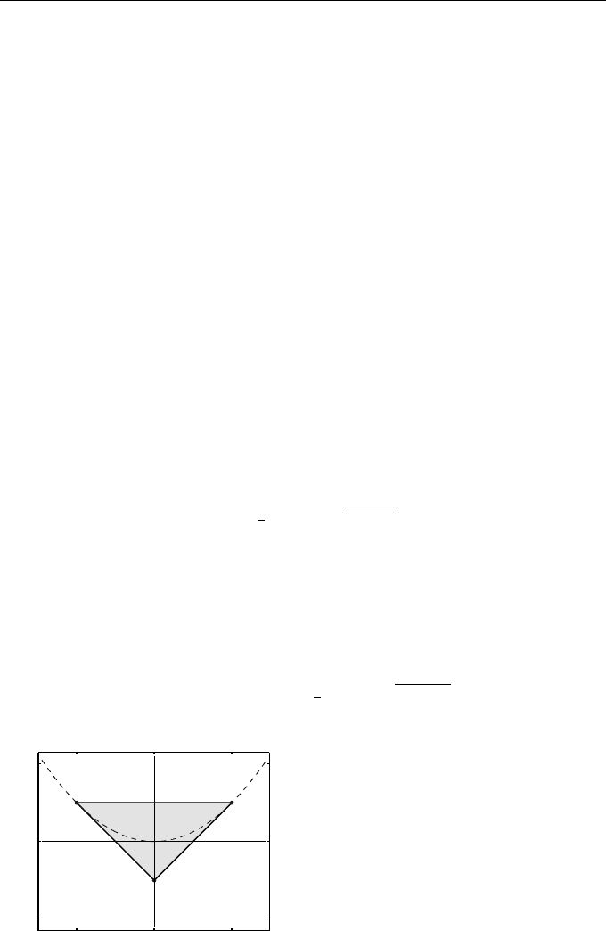
Lemma 6.10 (Ju ry Conditions)

The quadratic polynomial q(r) = r

+ ar + b, where a and b are both real

parameters, will satisfy the strict root condition of Deﬁnition 5.4 if, and only

if,

(i) b < 1, (ii) 1 + a + b > 0, and (iii) 1 − a + b > 0.

These are often called Jury conditions [40] and they deﬁne the triangular region

shown in Figure 6.8.

Proof

Using the quadratic formula, the roots of q(r) = r

+ ar + b are given by

, r



−a ±

− 4b



When a

< 4b the roots form a complex conjugate pair and, since b is equal

to the product of the roots, we ﬁnd that b = r

= |r

. Hence, the

strict root condition holds if, and only if, b < 1. The inequality a

< 4b also

implies that (ii) and (iii) are satisﬁed (see Exercise 6.4).

In the case of real roots (a

≥ 4b), the root of largest magnitude R is

R = max{|r

|, |r

|} =



|a| +

− 4b



−2 0 2

−2

b = 1

a +

−1

a −

(2, 1)(−2, 1)

Fig. 6.8 The interior of the shaded

triangle shows the points (a, b) where

the polynomial q(r) = r

+ ar + b sat-

isﬁes the s trict root conditions. (Solu-

tions are complex for values of a and b

above the broken line: b = a

/4)

6.2 Absolute Stability 85

This is an increasing function of |a|, and R = 1 when |a| = 1 + b. Hence,

0 ≤ R < 1 if, and only if, 0 ≤ |a| < 1 + b. Also, since the strict root condition

implies that |r

| < 1, it follows that |b| < 1 and condition (i) must hold.

Combining the res ults for real and complex roots, we ﬁnd that the strict

root condition is satisﬁed if, and only if, |a| − 1 < b < 1.

These conditions are equivalent to

q(0) < 1 and q(±1) > 0,

which may be easier to remember. To apply this lemma to the stability poly-

nomial (6.3) for a general two-step LMM it is ﬁrst necessary to divide by the

coeﬃcient of r

, so

a =

−

hβ

1 −

hβ

, b =

−

hβ

1 −

hβ

The denominators in these coeﬃcients are necessarily positive for all

h ∈ R

(see Exercise 6.12), so the conditions q(±1) > 0 can be replaced by p(±1) > 0.

For explicit LMMs, β

= 0 and q(r) will coincide with the stability polynomial

p(r).

Example 6.11

Find the interval of absolute stability of the LMM:

n+2

− x

n+1

= hf

The stability polynomial is quadratic in r:

p(r) = r

− r −

h; (6.4)

since

h is real, the coeﬃcients of this polynomial are real, and we can use

Lemma 6.10 to determine precisely when it satisﬁes the strict root condition.

Moreover, p(r) ≡ q(r), so the conditions for absolute stability are p(±1) > 0

and p(0) < 1. We ﬁnd

p(0) < 1 : −

h < 1 ⇒

h > −1,

p(1) > 0 : −

h > 0 ⇒

h < 0,

p(−1) > 0 : 2 −

h > 0⇒

h < 2.

In order to satisfy all three inequalities, we must have −1 <

h < 0. So the

interval of absolute stability is (−1, 0).