Griffiths D.F., Higham D.J. Numerical Methods for Ordinary Differential Equations: Initial Value Problems

Подождите немного. Документ загружается.

46 4. Linear Multistep Methods—I

Example 4.1

Apply the TS(2), trapezoidal and AB(2) methods to the IVP x

(t) = (1 −

2t)x(t), t ∈ (0, 4], x(0) = 1 (cf. Examples 2.1 and 3.1) with h = 0.2 and

h = 0.1. Compare the accuracy achieved by the various methods at t = 1.2.

The application of TS(2) is described in Example 3.1. With f(t, x) = (1 −

2t)x, the trapezoidal rule gives

n+1

= x

h[(1 − 2t

n+1

+ (1 − 2t

which can be rearranged to read

n+1

1 +

h(1 − 2t

)

1 −

h(1 − 2t

n+1

)

(4.11)

for n = 0, 1, 2, . . . and x

= 1. When h = 0.2 we take n = 6 steps to reach

t = 1.2, at which point we obtain x

= 0.789 47. Comparing this with the exact

solution x(1.2) = 0.786 63 gives a GE of −0.0028.

For the AB(2) method, we ﬁnd

n+2

= x

n+1

h[3(1 − 2t

n+1

− (1 − 2t

]



1 +

h(1 − 2t

n+1

)



n+1

−

h(1 − 2t

which holds for n ≥ 0. When n = 0 we have x

= 1, t

= 0, t

= h, and



1 +

h(1 − 2h)



−

It is necess ary to use some other method to ﬁnd the additional starting value

before we can begin. Two obvious possibilities are to use either Euler’s

method, x

= (1 + h)x

(we label the results ABE), or the value computed by

the trapezoidal rule (4.11) with n = 0 (leading to ABT).

The calculation of the sequence {x

} is best organized with a start-up phase:

ﬁrst calculate f

= 1 from the initial data x = x

at t = t

. The solution at

t = t

is then calculated by Euler’s method (for instance):

= t

+ h = 0.2,

= x

+ hf

= 1.2 (Euler’s method),

= (1 − 2t

= 0.72;

then, for each n = 0, 1, 2, . . . , x

n+2

and f

n+2

are calculated from

n+2

= t

n+1

+ h,

n+2

= x

n+1

h(3f

n+1

− f

n+2

= (1 − 2t

n+2

4.1 Introduction 47

0 1 2 3 4

0.2

0.4

0.6

0.8

1.2

0 1 2 3 4

−0.06

−0.05

−0.04

−0.03

−0.02

−0.01

0.01

0.02

TS(2)

Trap . R ule

AB(E )

AB(T)

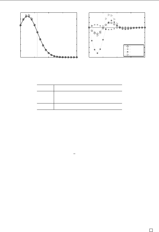
Fig. 4.1 Numerical solutions (left) and GEs (right) as functions of time with

h = 0.2 for Example 4.1

h TS(2) Trap. ABE ABT

0.2 5.4 −2.8 −3.6 17.6

0.1 1.4 −0.71 −0.66 4.0

Ratio 3.90 4.00 5.49 4.40

Table 4.1 Global errors (multiplied by 10

) at t = 1.2

so that the value of f at t = t

n+2

is available in the succeeding steps—i.e. the

value of f at any given grid point needs be computed only once.

The solutions obtained with these methods are shown in Figure 4.1 (left)

as functions of t

. These are indistinguishable from the exact solution curve

except near to the maximum at t =

; the corresponding GEs are shown in the

right of the ﬁgure. The GEs at t = 1.2 (obtained by subtracting the numerical

solutions from the exact solution) are shown in Table 4.1 for h = 0.2 and

h = 0.1. Dividing the GE when h = 0.2 by that when h = 0.1 leads to the

bottom row in Table 4.1. Since this ratio is close to 4, it suggests that the four

methods shown all converge at a second-order rate: e

∝ h

. Surprisingly, the

GE of ABE is smaller than that of ABT, which uses a more accurate starting

value x

. However, when we look at the behaviour of the GE over the whole

domain in Figure 4.1, we see that ABE has a particularly large GE at t ≈ 0.5;

to sample the errors at only one time may be misleading. Closer scrutiny of

the ﬁgure reveals that the greatest overall accuracy is given by the trapezoidal

rule, and we estimate that

TS(2)

≈ −GE

trap

, GE

ABT

≈ −2 GE

trap

, GE

ABE

≈ −5 GE

trap

48 4. Linear Multistep Methods—I

k p Method Name

1 1 x

n+1

− x

= hf

Euler

1 1 x

n+1

− x

= hf

n+1

Backward Euler

1 2 x

n+1

− x

h(f

n+1

+ f

) trapezoidal

2 2 x

n+2

− x

n+1

h(3f

n+1

− f

) two-step Adams–Bashforth

2 2 x

n+2

− x

n+1

h(5f

n+2

+ 8f

n+1

− f

) two-step Adams–Moulton

2 4 x

n+2

− x

h(f

n+2

+ 4f

n+1

+ f

) Simpson’s rule

2 3 x

n+2

+ 4x

n+1

− 5x

= h(4f

n+1

+ 2f

) Dahlquist (see Example 4.11)

Table 4.2 Examples of LMMs showing their step number (k) and order (p)

4.2 Two-Step Methods

So far we have encountered three examples of LMMs: Euler’s me thod, the

trapezoidal rule (4.7 ) and the AB(2) method (4.10). The last two were derived

from the expansions (4.3) and (4.9), which are valid for all three times diﬀer-

entiable functions z, and which we regard as being generalizations of Taylor

series—they relate the values of z and z

(t) at several diﬀerent points.

For the time being we shall be concerned only with two-step LMMs, such

as AB(2), that involve the three time levels t

, t

n+1

, and t

n+2

. For these, we

need to ﬁnd the coeﬃcients α

, α

, β

, and β

so that

z(t + 2h) + α

z(t + h) + α

z(t)

= h(β

(t + 2h) + β

(t + h) + β

(t)) + O(h

p+1

), (4.12)

where p might be speciﬁed in some cases or we might try to make p as large

as possible in others. We have taken α

= 1 as a normalizing condition (the

coeﬃcient of z(t + 2h)).

Choosing z = x, where x

= f (t, x), and dropping the O(h

p+1

) remainder

term, we arrive at the general two-step LMM

n+2

+ α

n+1

+ α

= h(β

n+2

+ β

n+1

+ β

). (4.13)

An LMM is said to be explicit (of explicit type) if β

= 0 and implicit if β

6= 0.

or example, Euler’s method (x

n+1

= x

+ hf

) is an example of an explicit

one-step LMM while the trapezoidal rule is an example of an implicit one-step

method.

On occasion we may write (4.13) in the form

n+2

+ α

n+1

+ α

= h(β

n+2

+ β

n+1

+ β

Some further examples of one- and two-step LMMs are listed in Table 4.2.

4.2 Two-Step Methods 49

4.2.1 Consistency

In order to streamline the process of determining the coeﬃcients in the LMM

(4.13), we introduce the notion of a linear diﬀerence operator.

Deﬁnition 4.2

The linear diﬀerence operator L

associated with the LMM (4.13) is deﬁned

for an arbitrary continuously diﬀerentiable function z(t) by

z(t) = z(t + 2h) + α

z(t + h) + α

z(t) −

h(β

(t + 2h) + β

(t + h) + β

(t)).

Apart from the remainder term, this is the diﬀerence between the left- and

right-hand sides of (4.12). L

is a linear operator since, for constants a and b,

(az(t) + bw(t)) = aL

z(t) + bL

w(t).

The construction of new methods amounts to ﬁnding suitable coeﬃcients

{α

, β

}. We shall prove later in this chapter that the coeﬃcients should be

determined so as to ensure that the resulting LMM is consistent.

Deﬁnition 4.3

A linear diﬀerence operator L

is said to be consistent of order p if

z(t) = O(h

p+1

)

with p > 0 for every smooth function z.

An LMM whose diﬀerence operator is consistent of order p for some p > 0 is

said to b e consistent. A method that fails to meet this requirement is called

inconsistent (see Exercise 4.9). This deﬁnition is in keeping with our ﬁndings

for TS(p) methods: an LTE of order (p + 1) gives rise to convergence of order

p (Theorem 3.2).

Example 4.4

Show that Euler’s method is consistent.

The linear diﬀerence operator for Euler’s method is

z(t) = z(t + h) − z(t) − hz

(t),

50 4. Linear Multistep Methods—I

which, by Taylor expansion, gives

z(t) =

(t) + O(h

and so L

z(t) = O(h

) and the method is consistent of order 1 (p = 1). 

Example 4.5

What is the order of consistency of the last method listed in Table 4.2?

The associated linear diﬀerence operator is

z(t) = z(t + 2h) + 4z(t + h) − 5z(t) − h(4z

(t + h) + 2z

(t)).

With the aid of the Taylor expansions

z(t + 2h) = z(t) + 2hz

(t) + 2h

(t) +

000

(t) +

0000

(t) + O(h

z(t + h) = z(t) + hz

(t) +

000

(t) +

0000

(t) + O(h

(t + h) = z

(t) + hz

(t) +

000

(t) +

0000

(t) + O(h

we ﬁnd (collecting terms appropriately)

z(t) = [1 + 4 − 5] z(t)

+ h [2 + 4 − [4 + 2]] z

(t)

+ h

[2 + 2 − 4] z

(t)

+ h



+ 4 ×

− 4 ×



000

(t)

+ h



+ 4 ×

− 4 ×



0000

(t) + O(h

Thus, L

z(t) =

0000

(t) + O(h

) and so L

z(t) = O(h

) and the method

is consistent of order p = 3. It is, in fact, the explicit two-step method having

highest possible order.

4.2.2 Construction

In the previous section the coeﬃcients of LMMs were given and we were then

able to ﬁnd their order and error constants. We now describe how the coeﬃ-

cients may be determined by the method of undetermined coeﬃcients.

For the general two-step LMM given by Equation (4.13) the associated

linear diﬀerence operator is (see Deﬁnition 4.2)

z(t) = z(t + 2h) + α

z(t + h) + α

z(t) −

h(β

(t + 2h) + β

(t + h) + β

(t)) (4.14)

4.2 Two-Step Methods 51

and the right-hand side may b e expanded with the aid of the Taylor expansions

z(t + 2h) = z(t) + 2hz

(t) + 2h

(t) +

000

(t) + . . . ,

z(t + h) = z(t) + hz

(t) +

000

(t) + . . . ,

(t + 2h) = z

(t) + 2hz

(t) + 2h

000

(t) +

0000

(t) + . . . ,

(t + h) = z

(t) + hz

(t) +

000

(t) +

0000

(t) + . . . .

The precise number of terms that should be retained depends on either the

order required

or the maximum order possible with the “template” used—

some coeﬃcients in the LMM may be set to zero in order to achieve a method

with a particular pattern of terms. It will also become clear as we proceed

that it is generally advantageous not to ﬁx all the coeﬃcients so as to achieve

maximum order of consistency, but to retain some free parameters to meet

other demands (notably stability).

We focus initially on the issue of consistency, i.e. what is needed for methods

to have order at least p = 1. Expanding the right of (4.14) we ﬁnd (collecting

terms appropriately)

z(t) =



1 + α

+ α



z(t) + h



2 + α

− (β

+ β

)



(t) + O(h

We shall have

z(t) = O(h

)

and, therefore, consistency of order 1, if the coeﬃcients are chosen so that

1 + α

+ α

= 0,

2 + α

= β

+ β

(4.15)

These conditions can be written more concisely if we introduce two poly-

nomials.

Deﬁnition 4.6

The ﬁrst and second characteristic polynomials of the LMM

n+2

+ α

n+1

+ α

= h(β

n+2

+ β

n+1

+ β

)

are deﬁned to be

ρ(r) = r

+ α

r + α

, σ(r) = β

+ β

r + β

(4.16)

respectively.

For order p all terms up to those containing h

p+1

must be retained but, since the

β-terms are already multiplied by h, the expansions of the z

terms need only include

terms up to h

52 4. Linear Multistep Methods—I

The following result is a direct consequence of Deﬁnition 4.3 and writing con-

ditions (4.15) in terms of the characteristic polynomials.

Theorem 4.7

The two-step LMM

n+2

+ α

n+1

+ α

= h(β

n+2

+ β

n+1

+ β

)

is consistent with the ODE x

(t) = f (t, x(t)) if, and only if,

ρ(1) = 0 and ρ

(1) = σ(1).

In general, when the right side of the linear diﬀerence operator (4.14) is

expanded to higher order terms and these are collected appropriately, it is

found that

z(t) = C

z(t) + C

(t) + ··· + C

(p)

(t) + O(h

p+1

), (4.17)

where, as in the lead up to (4.15), C

= 1 + α

+ α

and C

= 2 + α

− (β

+β

). The coeﬃcients C

are each linear combinations of the α and β values

that do not involve h. In view of Deﬁnition 4.3, an LMM will b e consistent of

order p if

= C

= ··· = C

= 0,

in which case

z(t) = C

p+1

(p+1)

(t) + O(h

p+2

). (4.18)

The ﬁrst non-zero coeﬃcient C

p+1

is known as the error constant.

The next theorem sheds light on the signiﬁcance of consistency.

Theorem 4.8

A convergent LMM is consistent.

Thus consistency is necessary for convergence, but it is not true to say that

consistent methods are always convergent.

Proof

Supp ose that the LMM (4.13) is convergent. Deﬁnition 2.3 then implies that

n+2

→ x(t

∗

+ 2h), x

n+1

→ x(t

∗

+ h) and x

→ x(t

∗

) as h → 0 when t

= t

∗

However, since t

n+2

, t

n+1

→ t

∗

, taking the limit on both sides of

n+2

+ α

n+1

+ α

= h(β

n+2

+ β

n+1

+ β

)

4.2 Two-Step Methods 53

leads to

ρ(1)x(t

∗

) = 0.

But x(t

∗

) 6= 0, in general, and so ρ

(1) = 0, the ﬁrst of the consistency conditions

in Theorem 4.7.

For the second part of the proof the limit h → 0 is taken of both sides of

n+2

+ α

n+1

+ α

= β

n+2

+ β

n+1

+ β

The right-hand side converges to the limit σ(1)f(t

∗

, x(t

∗

)) and, for the left-hand

side, we use the limits x

n+2

→ x(t

∗

+ 2h), x

n+1

→ x(t

∗

+ h), and x

→ x(t

∗

)

together with l’Hˆopital’s rule to conclude that

lim

h→0

n+2

+ α

n+1

+ α

= (2 + α

∗

Thus, the limiting function x(t) satisﬁes

(1)x

∗

) = σ(1)f(t

∗

, x(t

∗

))

at t = t

∗

, which is not the correct diﬀerential equation unless ρ

(1) = σ(1).

Example 4.9

Determine the coeﬃcients in the 1-step LMM

n+1

+ α

= h(β

n+1

+ β

)

so that the resulting method has order 1. Find the error constant and show

that there is a unique method having order 2. What is the error constant for

the resulting method?

The associated linear diﬀerence operator is, by deﬁnition,

z(t) = z(t + h) + α

z(t) − h(β

(t + h) + β

(t)) (4.19)

and Taylor expanding the terms z(t + h) and z

(t + h) gives

z(t) = (1 + α

)z(t) +



1 − (β

+ β

)



(t) + O(h

Therefore, we shall have consistency (i.e., order at least 1) if the terms in z(t)

and hz

(t) vanish. This will be the case if

1 + α

= 0 and 1 = β

+ β

The details are left to Exercise 4.17.

54 4. Linear Multistep Methods—I

These are two equations in three unknowns and their general solution may be

expressed as α

= −1, β

= θ, β

= 1−θ, which gives rise to the one-parameter

family of LMMs known as the θ-method:

n+1

− x

= h(θf

n+1

+ (1 − θ)f

). (4.20)

The error constant is C

, for which we have to retain one more term in each of

the Taylor expansions of z(t + h) and z

(t + h). We then ﬁnd

z(t) = (

− θ)h

(t) + O(h

)

so that C

− θ. The common choices for θ are:

1. θ = 0. Euler’s method: x

n+1

− x

= hf

2. θ = 1. Backward Euler method: x

n+1

− x

= hf

n+1

(see Table 4.2). This

is also known as the implicit Euler method.

3. θ =

. trapezoidal rule: x

n+1

− x

h(f

+ f

n+1

). This is the unique

value of θ for which C

= 0 and the me thod becomes of second order. To

compute its error constant C

, the Taylor expansions must be extended by

one term (with θ =

), so:

z(t) = h

(

−

θ)z

000

(t) + O(h

)

= −

000

(t) + O(h

)

and, therefore, C

= −

Example 4.10

Determine the coeﬃcients in the two-step LMM

n+2

+ α

= h(β

n+1

+ β

)

so that it has as high an order of consistency as possible. What is this order

and what is the error constant for the resulting method?

The associated linear diﬀerence operator is

z(t) = z(t + 2h) + α

z(t) − h(β

(t + h) + β

(t)).

The LMM contains three arbitrary constants so we expect to be able to sat-

isfy three linear equations; that is, we should be able to make the terms in

z(t), hz

(t), and h

(t) in the Taylor expansion of L

z(t) all vanish leaving

z(t) = C

000

(t) +O(h

). We therefore expect to have order p = 2; for this

to occur we have to retain terms up to h

000

(t). (For some methods we get a

“bonus” in that the next term is automatically z ero—see Simpson’s method.)

4.2 Two-Step Methods 55

With the aid of the Taylor series

z(t + 2h) = z(t) + 2hz

(t) + 2h

(t) +

000

(t) +

0000

(t) + O(h

)

(t + h) = z

(t) + hz

(t) +

000

(t) +

0000

(t) + O(h

)

we ﬁnd, on collecting terms in powers of h,

z(t) = [1 + α

] z(t) + h [2 − (β

+ β

)] z

(t)

+ h

[2 − β

] z

(t)

+ h



−



000

(t) + O(h

Setting the coeﬃcients of the ﬁrst three terms to zero gives

1 + α

= 0, 2 = β

+ β

, 2 = β

whose solution is α

= −1, β

= 2, β

= 0 and the resulting LMM is

n+2

− x

= 2hf

n+1

, (4.21)

known in some circles as the mid-point rule and in others as the “leap-frog”

method; we shall see in the next chapter that it belongs to the class of Nystr¨om

methods. It follows that

z(t) =

000

(t) + O(h

)

and so L

z(t) = O(h

) and the method is consistent of order p = 2 with error

constant C

An alternative approach to constructing LMMs based on interpolating poly-

nomials is suggested by Exercises 4.18 and 4.19.

Is this all there is to constructing LMMs? Theorem 4.8 did not say that

consistent methods are convergent, and the following numerical example indi-

cates that some further property is required to generate a useful (convergent)

method.

Example 4.11

Use the method

n+2

+ 4x

n+1

− 5x

= h(4f

n+1

+ 2f

)

(see Example 4.5) to solve the IVP x

(t) = −x(t) for t > 0 with x(0) = 1. Use

the three diﬀerent grid sizes h = 0.1, 0.001 and 0.0001 and, for the additional

starting value, use x

= e

−h