Griffiths D.F., Higham D.J. Numerical Methods for Ordinary Differential Equations: Initial Value Problems

Подождите немного. Документ загружается.

86 6. Linear Multistep Methods—III

Example 6.12

Find the interval of absolute stability of the mid-point rule: x

n+2

−x

= 2hf

n+1

In this case

p(r) = r

− 2

hr − 1,

whose roots are

h +

1 +

, r

−

h −

1 +

and it should be immediately obvious that |r

−

| > 1 when

h < 0, so the method

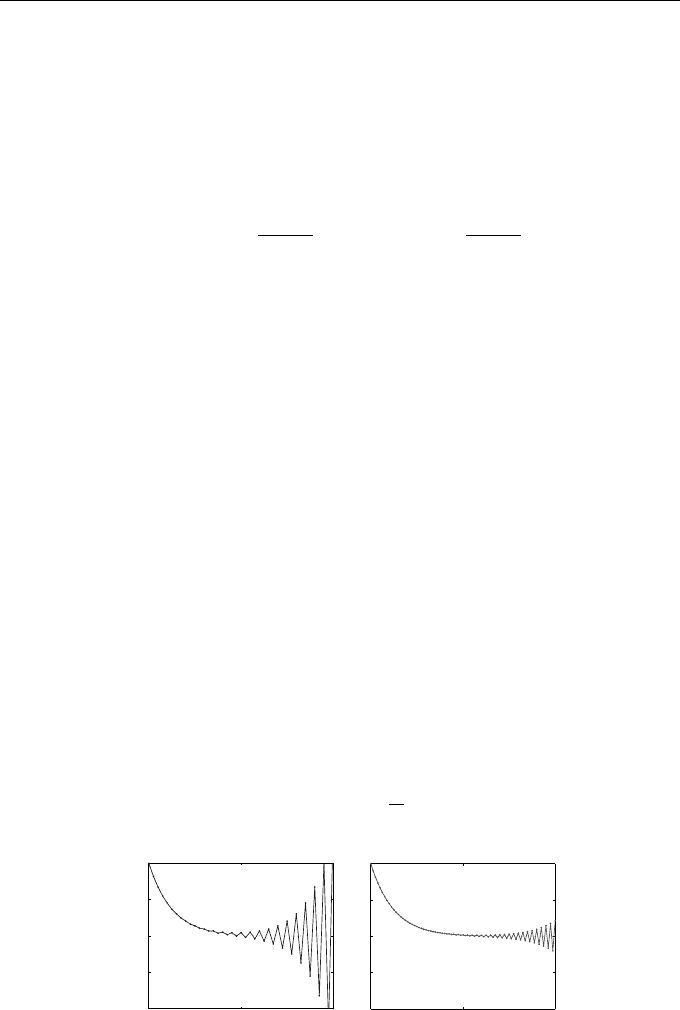
can never be absolutely stable. To see the consequences of this, the method

is applied to the IVP x

(t) = −8x(t) with x(0) = 1. The results are shown

in Figure 6.9 with h = 1/40 (

h = 1/5) and h = 1/120 (

h = 1/15) and the

additional starting value provided by the exact solution at t = t

. The solutions

of the mid-point rule are given by (the details are left to Exercise 6.13)

= Ar

+ Br

−

, (6.5)

where the constants A and B are chosen to satisfy the starting conditions

= 1, x

= e

. It can be shown that

= e

+ O(

) and r

−

= −e

−

+ O(

so that r

= e

λt

∗

+ O(h

) and r

−

= (−1)

−λt

∗

+ O(h

) at t

∗

= nh. The ﬁrst

of these approximates the corresponding term in the exact solution, e

λt

∗

, while

−

has no such role—for this reason it is usually referred to as a spurious root:

the ODE is of ﬁrst order but the diﬀerence equation that approximates it is of

second order. On solving for A and B and expanding the results in a Maclaurin

series in

h we ﬁnd

A = 1 + O(h

), B = −

+ O(h

0 0.5 1

−100

−50

100

0 0.5 1

−100

−50

100

Fig. 6.9 Numerical solution by the mid-point rule for Example 6.12 with

h = 1/40 (left) and h = 1/120 (right)

6.3 The Boundary Locus Method 87

Hence, the ﬁrst term Ar

in the solution (6.5) approximates the exact solution

to within O(h

) while the second term satisﬁes

−

= −

(−1)

−λt

∗

+ O(h

It is this term that causes problems: it is exponentially growing when <(λ) < 0

(and the exact solution is exponentially decaying) and the factor (−1)

causes

it to alternate in sign on consecutive steps (producing the oscillations evident

in Figure 6.9). On a positive note, it has an amplitude proportional to h

, so

becomes negligible compared with the dominant O(h

) term in the GE when

h is suﬃciently small.

Other Nystr¨om and Milne–Simpson methods have similar properties, so

cannot be recommended for solving problems with damping (<(λ) < 0). How-

ever, it is a diﬀerent story if λ is purely imaginary (oscillatory problems)—see

Section 7.3.

6.3 The Boundary Locus M ethod

It is, in general, quite diﬃcult to determine the region of absolute stability of an

LMM since we have to decide, for each

h ∈ C, whether the roots of the stability

polynomial satisfy the strict root condition (|r| < 1). It is more attractive to

look for the boundary of the region, because at least one of the roots of p(r)

on the boundary has modulus |r| = 1. Thus, the boundary is a subset of the

points

h ∈ C for which r = e

, where s ∈ R. Substituting r = e

into the

stability polynomial and solving for

h we obtain

h =

h(s) and plotting the

locus in the complex plane gives a curve, part of which will be the required

boundary. We illustrate the process with an example that contains most of the

important features.

Example 6.13

Use the boundary locus method to determine the boundary of the region of

absolute stability of the LMM x

n+2

− x

n+1

= hf

(see Example 6.11).

With r = e

the stability polynomial (6.4) gives

h = r

− r, and so

h(s) = e

2is

− e

= [cos(2s) − cos(s)] + i[sin(2s) − sin(s)].

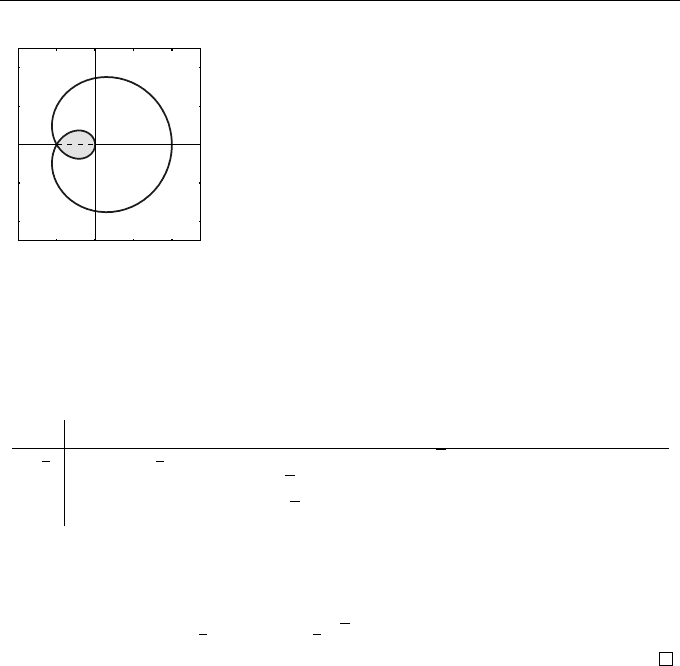
Plotting the locus of the points bx(s) = cos(2s) −cos(s), by(s) = sin(2s) −sin(s)

for 0 ≤ s < 2π we obtain the curve shown in Figure 6.10, which divides the

plane into three subregions—it remains to decide which subregion is the region

88 6. Linear Multistep Methods—III

−2 −1 0 1 2

−2

−1

ℜ(

ℑ(

Fig. 6.10 Stability region R for Example 6.13

(shaded). The solid curve is the locus of points

where the stability polynomial p(r) has at least one

root r with |r| = 1

of absolute stability. We need only test one point in each subregion: if the roots

at that point satisfy the strict root condition then the point lies in the region

of absolute stability, otherwise it does not lie in the region. This is done in the

table below.

h p(r) Roots |r| Absolutely stable

−

− r +

r = (1 ± i)/2 |r| = 1/

√

2 < 1 yes

1 r

− r − 1 r = (1 ±

√

5)/2 |r| > 1 no

−2 r

− r + 2 r = (1 ± i

√

7)/2 |r| > 1 no

We conclude that the region of absolute s tability is the shaded region in

Figure 6.10. The curve intersects itself when =(

h(s)) = 0. This is easily s hown

to occur when cos s =

, so sin s =

√

3 and

h = −1. The interval of absolute

stability is, therefore, (−1, 0), in agreement with Example 6.11.

6.4 A-stability

Some LMMs (the trapezoidal rule is one example) applied to the mo del prob-

lem (6.1) have the satisfying property that x

→ 0 as n → ∞ whenever

x(t) → 0 as t → ∞ regardless of the size of h. This is suﬃciently important to

give the set of all such methods a name:

Deﬁnition 6.14 (A-Stability)

A numerical method is said to be A-stable if its region of absolute stability R

includes the entire left half plane (<(

h) < 0).

This is a severe requirement, as evidenced by the following theorem.

6.4 A-stability 89

Theorem 6.15 (Dahlquist’s Second Barrier Theorem)

1. There is no A-stable explicit LMM.

2. An A-stable (implicit) LMM cannot have order p > 2.

3. The order-two A-stable LMM with scaled error constant (C

p+1

/σ(1)) of

smallest magnitude is the trapezoidal rule.

Proof

See Hairer and Wanner [29].

We can relax our requirements when λ is real.

Deﬁnition 6.16 (A

-Stability)

A numerical method is said to be A

-stable if its interval of absolute stability

includes the entire left real axis (<(

h) < 0, =(

h) = 0).

As a parting remark, we observe that A-stability has been deﬁned in terms of

the simple linear diﬀerential equation x

(t) = λx(t). What is remarkable (and

not fully understood) is why methods which are A-stable generally outperform

other methods on more general non-linear problems.

EXERCISES

6.1.

By writing

h = 2X + 2iY in Example 6.9 prove that

− 1 =

(1 − X)

+ Y

and deduce that |r

| < 1 for all <(

h) < 0.

What can be concluded about the interval of absolute stability of

the trapezoidal rule?

6.2.

Prove that the region of absolute stability of the backward Euler

method x

n+1

= x

+ hf

n+1

is given by |1 −

h| > 1. By writing

h = bx + iby show that this corresponds to the exterior of the circle

(bx − 1)

+ by

= 1. Sketch a diagram analogous to Figure 6.6.

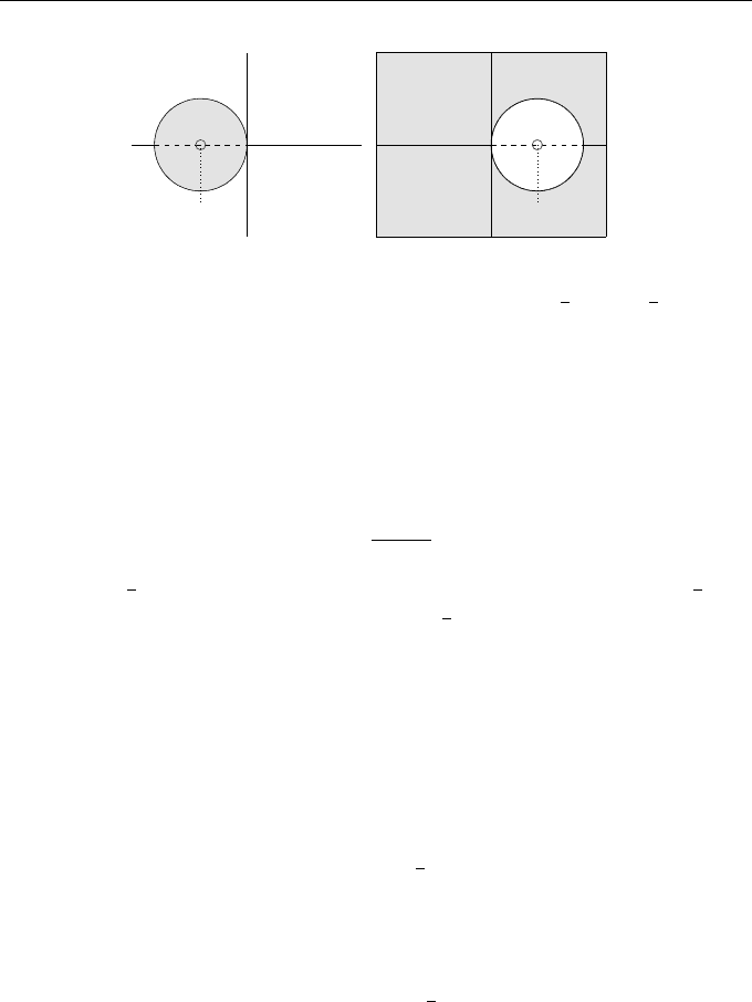
90 6. Linear Multistep Methods—III

ℜ(

ℑ(

bx = 1/(2θ − 1)

ℜ(

ℑ(

bx = 1/(2θ − 1)

Fig. 6.11 The region of absolute stability for the θ-method (shaded) and the

interval of absolute stability (broken line). Left: 0 ≤ θ <

; right:

< θ ≤ 1.

See Exercise 6.3.

6.3.

Determine the region of absolute stability of the θ-method

n+1

− x

= h(θf

n+1

+ (1 − θ)f

By writing

h = bx + iby show that this corresponds to the exterior of

the circle

2θ − 1

bx + by

= 0

< θ ≤ 1 and to the interior of the circle if 0 ≤ θ <

. See

Figure 6.11. What happens at θ =

6.4.

Verify the identity

− 4b = (|a| − 2)

− 4



1 + b − |a|



for any real numbers a, b and deduce that b > |a| − 1 whenever

< 4b, as required in the proof of Lemma 6.10.

6.5.

Find the interval of absolute stability of the LMM

n+2

− x

h(f

n+1

+ 3f

6.6.

Find the interval of absolute stability of the two-step Adams–

Bashforth method (AB(2))

n+2

− x

n+1

h(3f

n+1

− f

6.7.

Consider the one-parameter family of LMMs

n+2

− 4θx

n+1

− (1 − 4θ)x

= h



(1 − θ)f

n+2

+ (1 − 3θ)f



for solving the ODE x

(t) = f (t, x), where the notation is standard.

(a) Determine the error constant for this family of methods and

identify the method of highest order. What is its error constant?

Exercises 91

−2 −1 0

−1

ℜ(

ℑ(

−8 −6 −4 −2 0 2

−4

−3

−2

−1

ℜ(

ℑ(

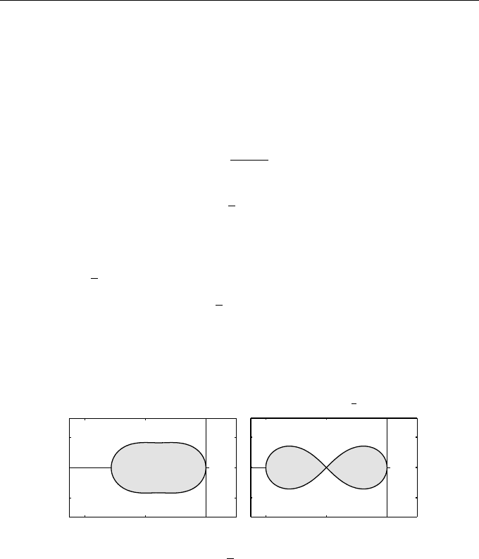
Fig. 6.12 Stability regions R for Exercise 6.9. One belongs to the Adams–

Bashforth method AB(2) and the other to the Adams–Moulton method AM(2)

(b) For what values of θ are members of this family of methods

convergent?

Is the method of highest order convergent? Explain your answer

carefully.

-stable when θ = 1/4.

6.8.

???

What is the stability polynomial of the LMM

n+2

− (1 + a)x

n+1

+ ax

h[(5 + a)f

n+2

+ 8(1 − a)f

n+1

− (1 + 5a)f

– Why must the condition −1 ≤ a < 1 be stipulated?

– Assuming that

h ∈ R, show that the discriminant of the (quadratic)

stability p olynomial is strictly positive for all values of

h and a.

What information does this give regarding its roots?

– Deduce that the interval of absolute stability is (−6

1+a

1−a

, 0).

6.9.

Shown in Figure 6.12 are the stability regions of the AB(2) (see

Exercise 6.6) and the Adams–Moulton method (AM(2))

n+2

− x

n+1

h(5f

n+2

+ 8f

n+1

− f

). (6.6)

Use the boundary locus method to ascertain which region belongs

to which method.

6.10.

Apply the boundary locus me thod to the mid-point rule (see Exam-

ple 6.12) to show that

h(s) = i sin s

so that the region of absolute stability consists of that part of the

imaginary axis between −i and i.

92 6. Linear Multistep Methods—III

6.11.

Show that the LMM

n+2

− x

n+1

h(f

n+2

+ 2f

n+1

+ f

)

is A

-stable.

6.12.

Prove that the coeﬃcient of r

in the stability polynomial (6.3) is

always positive for

h in the interval of absolute stability; i.e.

1 −

hβ

> 0 for all

h ∈ R

6.13.

???

Complete the details in Example 6.12. Show, in particular, that

A =

(1 + a) and B =

(1 − a), where

a =

−

1 +

= 1 +

+ O(

Deduce that A = 1 + O(

) and B = O(

6.14.

Find the interval of absolute stability of each member of the con-

vergent family of LMMs of the form (see Exercise 5.11)

n+2

− x

= h (β

n+1

+ β

Why can no member of the family be identiﬁed as having the largest

such interval?

6.15.

???

Show that all convergent members of the family of methods

n+2

+ (θ − 2)x

n+1

+ (1 − θ)x

h [(6 + θ)f

n+2

+ 3(θ − 2)f

parameterized by θ, are also A

-stable.

6.16.

Show that the method

n+2

− 3x

n+1

+ x

h (4f

n+2

− 3f

n+1

+ f

)

is A

-stable.

6.17.

???

Consider the family of LMMs

n+2

− 2ax

n+1

+ (2a − 1) x

= h [af

n+2

+ (2 − 3a) f

n+1

where a is a parameter.

(a) What are its ﬁrst and sec ond characteristic polynomials?

(b) When is the method consistent?

Exercises 93

(d) When is the method convergent?

(e) What is its order? What is the error constant?

(f) Are there any members of the family that are A

-stable?

(g) What c onclusions can you draw concerning the backward diﬀer-

entiation formula (BDF(2))

n+2

− 4x

n+1

+ x

= 2hf

n+2

(h) Verify that all three statements of Dahlquist’s second barrier

theorem hold for this family of methods.

6.18.

Show that the method 2x

n+2

− x

n+1

− x

= 3hf

n+2

is A

-stable.

Use the b oundary locus method to show that, on the boundary of

the region of stability,

h(s) = (2 − e

−is

− e

−2is

)/3. Deduce that

h(s)) ≥ 0 for all s and conclude that the method is A-stable.

6.19.

Use Lemma 6.10 to derive necessary and suﬃcient conditions on

the (real) coeﬃcients (a, b) for the roots of the polynomial q(r) =

+ ar + b to satisfy the root condition. Pay particular attention to

double roots having m odulus equal to one.

6.20.

???

Supp ose that a convergent LMM has a cubic characteristic poly-

nomial

ρ(r) = r

+ ar

+ br + c.

Prove that

(a) it can be factorized as ρ(r) = (r − 1)(r

+ (1 + a)r − c);

(b) the coeﬃcients a and c must satisfy

2 + a − c > 0, a + c ≤ 0, 1 + c ≥ 0

while excluding the point (a, c) = (1, −1).

[Hint: use Lemma 6.10, paying particular attention to roots of

ρ(r) with |r| = 1.]

6.21.

???

The composite Euler method uses Euler’s method with a step size

on even-numbered steps and a step size h

on odd-numbered

steps, so

2m+1

= x

+ h

and x

2m+2

= x

2m+1

+ h

2m+1

where h

= (1 − γ)h, h

= (1 + γ)h (0 ≤ γ < 1) so a time interval

of 2h is covered in two consecutive steps. The interval of absolute

94 6. Linear Multistep Methods—III

stability of this composite method can be deduced by applying it to

the ODE x

(t) = λx(t) and examining the ratio R(

h) = x

2m+2

Show that R(

h) = (1 +

− γ

By determining the global m inimum of the function R(

h), prove

that −1 < R(

h) < 1 if, and only if,

h lies in the interval of absolute

stability given by

−

1 − γ

h < 0.

Deduce that the largest interval of absolute stability is

h ∈ (−4, 0)

and occurs when γ = 1/

√

2. Hence, the composite method may be

used in a stable manner with a value of h that is twice as large as the

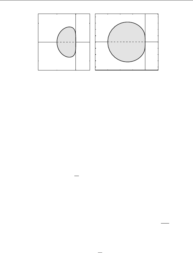
standard Euler method. The region of absolute stability with γ = 0

is the same as for Euler’s method (Figure 6.8); when γ = 3/5 and

√

2 it is as shown in Figure 6.13.

6.22.

Supp ose that γ = 1/

√

2 and λ = −8 + i in the previous exercise.

Show that the method will be absolutely s table when h = 1/8 and

3/8 but not when h = 1/4 and 1/2. Relate these results to the region

of absolute stability shown in Figure 6.13. See also Exercise 10.14.

−4 −2 0

−1

γ = 3/5

ℜ(

ℑ(

−4 −2 0

−1

γ = 1/

√

ℜ(

ℑ(

Fig. 6.13 The region of absolute stability for the composite Euler method for

Exercise 6.21 when γ = 3/5 and 1/

√

Linear Multistep Methods—IV:

Systems of ODEs

In this chapter we describe the use of LMMs to solve systems of ODEs and

show how the notion of absolute stability can be generalized to such problems.

We begin with an example.

Example 7.1

Use the LMM (AB(2))

n+2

− x

n+1

h(3f

n+1

− f

)

to compute the solution at t = 0.2 of the IVP

(t) = −tu(t)v(t),

(t) = −u

(t),

with u = 1, v = 2 at t = 0. Use h = 0.1 and Euler’s method to calc ulate u

and v

We begin by using the diﬀerential equations to calculate u

(0) = 0 and

(1) = −1 so we have the starting values

= 0, u

= 1, v

= 2, u

= 0, v

= −1.

Springer Undergraduate Mathematics Series, DOI 10.1007/978-0-85729-148-6_7,

D.F. Griffiths, D.J. Higham, Numerical Methods for Ordinary Differential Equations,