Griffiths D.F., Higham D.J. Numerical Methods for Ordinary Differential Equations: Initial Value Problems

Подождите немного. Документ загружается.

116 8. Linear Multistep Methods—V

` 0 1 2 3

[`]

1.00 0.774 647 887 0.773 901 924 0.773 901 807

1.00 1.042 253 521 1.041 731 347 1.041 731 265

[`]

2.2535 × 10

−1

7.4596 × 10

−4

1.1711 × 10

−7

2.9131 × 10

−15

−4.2254 × 10

−2

5.2217 × 10

−4

8.1975 × 10

−8

1.9628 × 10

−15

[`]

2.2610 × 10

−1

7.4608 × 10

−4

1.1711 × 10

−7

2.8866 × 10

−15

−4.1731 × 10

−2

5.2226 × 10

−4

8.1975 × 10

−8

1.9984 × 10

−15

Table 8.2 Results illustrating convergence of the Newton–Raphson iteration

to determine x

in Example 8.15

The Jacobian of F (u) is given by

∂F

∂x

(u) =



1 6hv

−2h 1 + 3hv



so a typical iteration of the Newton–Raphson method involves solving



1 6h(v

[`]

)

−2h 1 + 3h(v

[`]

)



[`]

= F (u

[`]

)

and then setting u

[`+1]

= u

[`]

−

[`]

, for ` = 0, 1, 2, . . . with u

[0]

= [1, 1]

. The

results are summarized in Table 8.2. Not only have we shown more iterations

than nec es sary, we have also included more digits in each entry than the accu-

racy of the method warrants. This has been done to fully illustrate how rapidly

convergence occurs and to show that convergence is indeed quadratic (see Ex-

ercise 8.13). The last two rows of the table have been computed by preforming

two further iterations and regarding the result as being the exact solution to

(8.16). It is also seen from Table 8.2 that

[`]

≈ E

[`]

—this is a consequence

of the rapid convergence. Since the underlying method is only ﬁrst-order ac-

curate and the grid size h = 0.1 is quite large, the ﬁrst iterate u

[1]

is already

suﬃciently accurate.

8.5 Postscript

The eﬃcient treatment of implicit methods is an essential requirement for deal-

ing with stiﬀ systems of ODEs. We have given an introduction to the basic ideas,

but further reﬁnements are common. For example, using an explicit LMM as

a predictor will generally provide a better starting value for ﬁxed-point itera-

tions. Also, at the end of Section 8.2 it was shown in (8.9) that u

[`+1]

− u

[`]

was equal to the residual when u = u

[`]

was substituted into the implicit LMM.

8.5 Postscript 117

−0.5 0 0.5 1

−1

−0.5

0.5

1.5

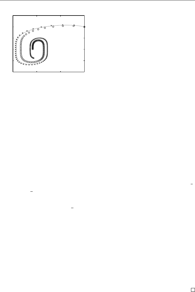
Fig. 8.1 Numerical solutions for Ex-

ample 8.3 integrated over 0 ≤ t ≤

10. The circles show the solution with

backward Euler and the crosses the so-

lution with local extrapolation, both

with h = 0.1. The solid curve shows

an accurate s olution computed with an

RK method

Recalling that the LTE is obtained when the exact solution is substituted into

the same equation, it makes sense for the iteration process to be terminated

when u

[`+1]

− u

[`]

is of the same magnitude as the LTE. The predicted value

can then be used, via Milne’s device, to estimate the LTE.

The idea of using an explicit predictor with Milne’s device can also be used

with the Ne wton–Raphson method. In Example 8.3, the use of Euler’s method

to predict a value of x

would give

[0]

= x

+ hf (t

, x

) =



0.8

1.1



The earlier use of the Newton–Raphson iteration to solve the backward Euler

equations gave x

= [0.7739, 1.0417]

(see Table 8.2) and these two approxima-

tions can be combined in Milne’s device (Equation (8.11) with p = 1, C

∗

and C

= −

) to give the LTE estimate

−

− x

[0]

) =



0.013

0.029



For local extrapolation this is added to the backward Euler solution to give

the updated solution x

= [0.7752, 1.0707]

which lies much clos er to the exact

solution x(t

) = [0.7757, 1.0661]

(to four decimal places).

The s ystem is now integrated over the time interval 0 ≤ t ≤ 10 and the

resulting phase plane solutions are shown in Figure 8.1. The numerical solution

using the backward Euler method is shown by circles (◦), the solution with local

extrapolation by crosses (×), and an accurate numerical solution (computed

with the Mat lab command ode45) as a solid curve. The extrapolated solution,

which was obtained with little additional computational cost, is signiﬁcantly

more accurate than the backward Euler solution.

118 8. Linear Multistep Methods—V

EXERCISES

8.1.

Solve the quadratic equation (8.7) for x

n+1

in terms of x

and h.

Discuss the behaviour of these solutions as h → 0.

8.2.

Extend the calculation in Example 8.2 to determine x

. What is the

improved value given by Milne’s device?

8.3.

Calculate E

[`]

(= u

[`]

− x

) for the data in Table 8.1 for ` = 0 : 3

on the basis that x

= 0.236 07. Show that these values have the

property that E

[`+1]

[`]

is approximately constant and the value

of this constant is approximately hB, where B is an appropriate

Jacobian evaluated at x = x

, thus conﬁrming the approximation

(8.6). Deduce that successive iterates gain approximately one extra

digit of accuracy.

8.4.

Apply the backward Euler method with h = 0.1 to solve the IVP de-

scribed in Example 8.3. Calculate the ﬁrst two ﬁxed-point iterations

in the determination of x

from a starting guess of u

[0]

= x

8.5.

For the system of ODEs in Example 8.3, show that



x(t)

y(t)



= −2y(t)

The quantity V (t) ≡ x(t)

y(t)

is an example of a Lyapunov

function. Its time derivative is negative e xcept when y(t) = 0, in

which case, x

(t) = 0 and y

(t) = 2x(t)—so the motion is vertical and

counterclockwise in the phase plane. V (t) is therefore a decreasing

function of t, from which it can be concluded that, in the long term,

the solution spirals to the origin.

8.6.

Apply the forward and backward Euler methods as a predictor-

corrector pair to approximate x

for the IVP described in Exam-

ple 8.3 with h = 0.1. Compare your answers with those given in

Table 8.2.

Use Milne’s device to produce a revised estimate of the solution at

t = t

8.7.

Apply the forward and backward Euler methods as a predictor-

corrector pair to solve the model equation x

(t) = λx(t) and show

that

n+1

= (1 +

h +

where

h = hλ. Hence, show that the interval of absolute stability of

this method is

h ∈ (−1, 0). The region of absolute stability is shown

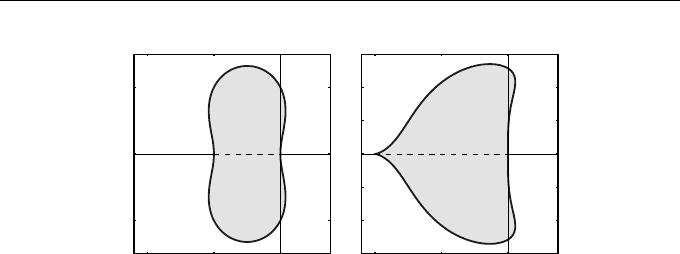
in Figure 8.2 (left).

Exercises 119

−2 −1 0

−1

ℜ(

ℑ(

−2 −1 0

−1.5

−1

−0.5

0.5

1.5

ℜ(

ℑ(

Fig. 8.2 The region of absolute stability for the forward/backward Euler

PECE method for Exercise 8.7 (left) and the AB(2)/trapezoidal pair for Exer-

cise 8.15 (right)

8.8.

(Based on Stuart and Humphries [65, page 270].) Applying the back-

ward Euler method to the ODE x

(t) = −x

(t) requires us to ﬁnd a

root of the cubic equation g(u) = u − x

+ hu

. Show that, for any

ﬁxed h > 0 and x

(i) g(u) → −∞ as u → −∞;

(ii) g(u) → ∞ as u → ∞;

(iii) g(u) is monotonically increasing.

Deduce that there is always a unique solution for the backward Euler

method in this case.

This example is studied further in Exercise 14.12.

8.9.

The scalar function f is said to satisfy a one-sided Lipschitz con-

dition if there exists a constant γ such that, for all u, v,

(u − v)(f(u) − f(v)) ≤ γ(u − v)

Consider applying backward Euler to the ODE x

(t) = f(x). Show

that when f satisﬁes a one-sided Lipschitz condition there is always

a unique solution if hγ < 1. In particular, this implies that there

is a unique solution for any step size when γ ≤ 0. (Hint: if there

are two distinct solutions, u and v, then u = x

+ hf(u) and v =

+hf(v). Subtract one equation from the other, multiply both sides

by u − v and apply the one-sided Lipschitz condition.) These ideas

can be generalized for systems of ODEs; see, for example, Stuart and

Humphries [65].

8.10.

Following on from Exercises 8.8 and 8.9, show that f(u) = −u

satisﬁes a one-sided Lipschitz condition with γ = 0. Also show that

120 8. Linear Multistep Methods—V

f(u) = u − u

satisﬁes a one-sided Lipschitz condition and, hence,

ﬁnd a condition on h that guarantees a unique solution for backward

Euler applied to x

(t) = x(t) − x

(t).

8.11.

Use the Newton–Raphson m ethod to solve Equation (8.8) with

[0]

= 0.2. How many iterations are required so that |u

[`+1]

−u

[`]

| <

0.001?

8.12.

Use the AB(2) and trapezoidal methods

n+2

= x

n+1

h(3f

n+1

− f

), C

∗

n+2

= x

n+1

h(f

n+2

+ f

n+1

), C

= −

as a predictor-corrector pair to calculate x

for the IVP of Exam-

ple 8.1 with h = 0.1 and the extra starting value x

= 0.233 922. Use

the error constants shown above with Milne’s device to es timate the

LTE at the end of this step and incorporate this to ﬁnd a higher or-

der approximation to x

. How do these two solutions compare with

the exact solution x(t

) = 0.271 645 (to six decimal places).

This process is generalized in Exercise 11.13 to variable step sizes.

8.13.

Supp ose that E

[`]

= [p

[`]

, q

[`]

]

. Use the data provided in the last

two rows of Table 8.2 to show that

[`]

)

[`+1]

≈ 4.75

for ` = 1, 2, thus conﬁrming quadratic convergence. Show that a

similar result holds for the second component q

[`]

8.14.

Write down the equations that have to be solved when the trape-

zoidal rule is used to compute an approximation to x(t

) for the

IVP described in Example 8.3 with h = 0.1. Carry out two iter-

ations when the Newton–Raphson method is used to solve these

equations starting from the initial guess x(0) = [1, 1]

. How does

the numerical solution at this stage compare with the values ob-

tained in Exercise 8.6 from the backward Euler method with and

without local extrapolation?

8.15.

???

Show that the PECE pair comprising AB(2) and trapezoidal meth-

ods of Exercise 8.12 applied to ODE x

(t) = λx(t) leads to

n+2

= (1 +

h +

n+1

−

Hence, show that the the interval of absolute stability of this method

h ∈ (−2, 0). The region of absolute stability is shown in Figure 8.2

(right).

Exercises 121

8.16.

Supp ose that C is a positive c onstant, −1 < r < 1, and v a unit

vector. The sequence E

[`]

= Cr

v converges geometrically to zero

(behaviour typical of ﬁxed-point iterations). Show that

[`+1]

− E

[`]

k = (1 − r)kE

[`]

and so the distance to the limit is given by

[`]

k =

1 − r

when kE

[`+1]

−E

[`]

k = ε. Thus, when the iteration is slowly conver-

gent (r is close to, but smaller than, unity), the distance from the

limit may be considerably further than the distance b etween suc-

cessive iterates. Thus, to ensure that kE

[`]

k < δ, iterations should

continue until kE

[`+1]

− E

[`]

k < (1 − r)δ.

8.17.

Using the values of E

[`]

and r = hB calculated in Exercise 8.3, verify

that the data in Table 8.1 satisfy (approximately) the result

[`]

| =

[`+1]

− E

[`]

1 − r

that was derived in the previous exercise.

8.18.

It was shown in Section 5.4 that, for linear ODEs, the leading term

in the LTE for both explicit and implicit two-step LMMs was equal

to the diﬀerence between the computed approximation ex and the

exact solution x(t

n+2

), under the localizing assumption that all back

values are exact. This result holds more generally and, updating the

notation to match the predictor-corrector setting, we have, under

the localizing assumption,

P: x(t

n+k

) − x

[0]

n+k

= T

∗

n+k

= h

p+1

∗

p+1

n+k

)

C: x(t

n+k

) − x

n+k

= T

n+k

+ O(h

p+2

)

= h

p+1

n+k

) + O(h

p+2

By ignoring higher order terms, express h

p+1

(p+1)

n+k

) in terms

of x

[0]

n+k

and x

n+k

. Hence, show that the leading term in T

n+k

given by (8.11).

Runge–Kutta Method—I:

Order Conditions

9.1 Introductory Examples

Runge–Kutta (RK) m ethods are one-step methods composed of a number of

stages. A weighted average of the slopes (f ) of the solution computed at nearby

points is used to determine the solution at t = t

n+1

from that at t = t

. Euler’s

method is the simplest such method and involves just one stage.

As in earlier chapters, we will develop methods for s olving the IVP

(t) = f (t, x(t)), t > t

x(t

) = η



. (9.1)

We give two examples of RK methods before going on to describe the general

method.

Example 9.1 (An Explicit RK Method)

Use the two-stage RK method (known as the “modiﬁed Euler method”) given

= f(t

, x

= f(t

h, x

n+1

= x

+ hk

n+1

= t

+ h

Springer Undergraduate Mathematics Series, DOI 10.1007/978-0-85729-148-6_9,

D.F. Griffiths, D.J. Higham, Numerical Methods for Ordinary Differential Equations,

124 9. Runge–Kutta Method—I: Order Conditions

to calculate approximate solutions to the IVP (see Example 2.1)

(t) = (1 − 2t)x(t), t > 0,

x(0) = 1

(9.2)

at t = h and t = 2h using h = 0.2.

We ﬁnd that

= f(t

, x

) = (1 − 2t

= f(t

h, x

)

= (1 − 2t

− h)(x

So, with h = 0.2:

n = 0 : k

= (1 − 2t

= 1,

= (1 − 2t

− h)(x

) = 0.8(1.1) = 0.88,

= x

+ hk

= 1.176,

= t

+ 0.2 = 0.2.

n = 1 : k

= (1 − 2t

= 0.6 × 1.176 = 0.7056,

= (1 − 2t

− h)(x

) = 0.498 62,

= x

+ hk

= 1.176 + 0.2 × 0.498 62 = 1.2757,

= t

+ 0.2 = 0.4.

This is an example of an explicit RK method: each k can be calculated without

having to solve any equations. When the calculations are extended to t = 1.2

and repeated with h = 0.1 we ﬁnd the GEs shown in the ﬁnal column of

Table 9.1. The GEs for this method are comparable with those from the second-

order methods of earlier chapters.

h TS(2) Trap. ABE ABT RK(2)

0.2 5.4 −2.8 −3.6 17.6 3.5

0.1 1.4 −0.71 −0.66 4.0 0.67

Ratio 3.90 4.00 5.49 4.40 5.24

Table 9.1 Global errors (multiplied by 10

) at t = 1.2 for the RK(2) method of

Example 9.1 alongside the GEs for the second-order methods used in Table 4.1

9.2 General RK Metho ds 125

Example 9.2 (An Implicit RK Method)

For the implicit RK method deﬁned by

= f(t

+ (

− γ)h, x

+ (

− γ)hk

= f(t

+ (

+ γ)h, x

+ (

+ γ)hk

n+1

= x

h(k

+ k

where γ =

√

3/6, determine x

n+1

in terms of x

when applied to the IVP

(t) = λx(t) with x(0) = 1.

With f(t, x) = λx, we obtain

= λ(x

+ (

− γ)hk

= λ(x

+ (

+ γ)hk

Writing

h = hλ, these equations may be rearranged to read

1 −

h −(

− γ)

−(

+ γ)

h 1 −









λx

, (9.3)

which may be solved for k

and k

. It may then be shown that (see Exer-

cise 9.10)

n+1

1 +

h +

1 −

h +

. (9.4)

Implicit RK methods are obviously much more complicated than both their

explicit versions and corresponding LMMs. The complexity can be justiﬁed

by improved stability and higher order: the method described in the previous

example is A-stable and of fourth-order (see Exercises 9.10 and 10.13).

9.2 General RK Methods

The general s-stage RK method may be written in the form

n+1

= x

+ h

i=1

, (9.5)

where the {k

} are computed from the function f :

= f





+ c

h, x

+ h

j=1

i,j





, i = 1 : s. (9.6)