Griffiths D.F., Higham D.J. Numerical Methods for Ordinary Differential Equations: Initial Value Problems

Подождите немного. Документ загружается.

6 1. ODEs—An Introduction

Example 1.3 (Lotka–Volterra Equations)

The Lotka–Volterra equations (developed circa 1925) oﬀer a simplistic model of

the conﬂict between populations of predators and prey. Suppose, for instance,

that the numbers of rabbits and foxes in a certain region at time t are u(t) and

v(t) respectively. Then, given the initial population siz es u(0) and v(0) at time

t = 0, their numbers might evolve according to the autonomous system

(t) = 0.05u(t)



1 − 0.01v(t)



(t) = 0.1v(t)



0.005u(t) − 2



(1.10)

These ODEs reproduce certain features that make sense in this predator-prey

situation. In the ﬁrst of these:

– Increasing the number of foxes (v(t)) decreases the rate (u

(t)) at which

rabbits are produced (because more rabbits get eaten).

– Increasing the number of rabbits (u(t)) increases the rate at which rabbits

are produced (because more pairs of rabbits are available to mate).

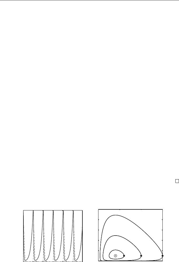
The solutions corresponding to an initial population of 1500 rabbits (solid

curves) and 100 foxes (dashed curves) are shown on the left of Figure 1.3.

On the right we plot these, and other solutions, in the phase plane, i.e., the

locus of the point (u(t), v(t)) parameterized by t for 0 ≤ t ≤ 600. Initially there

are 100 foxes and the three curves corresp ond to there being initially 600, 1000,

and 1500 rabbits (the starting values are shown by solid dots). The periodic

nature of the p opulations can be deduced from the fact that these are closed

curves. The “centre” of rotation is indicated by a small circle.

The text by Murray [56] is packed with examples where ODEs are used to

model biological processes.

0 100 200 300 400 500 600

500

1000

1500

u(t), v (t)

0 500 1000 1500

200

400

600

800

1000

u(t)

v(t)

Fig. 1.3 Solutions for the Lotka–Volterra equations (1.10)

1.1 Systems of ODEs 7

Example 1.4 (Biochemical Reactions)

In biochemistry, a Michaelis–Menten-type process involving

– a substrate S,

– an enzyme E,

– a complex C, and

– a product P

could be summarized through the reactions

S + E

→ C

→ S + E

→ P + E.

In the framework of chemical kinetics, this set of reactions may be interpreted

as the ODE system

(t) = −c

S(t) E(t) + c

C(t),

(t) = −c

S(t) E(t) + (c

+ c

)C(t),

(t) = c

S(t) E(t) − (c

+ c

)C(t),

(t) = c

C(t),

where S(t), E(t), C(t) and P (t) denote the concentrations of substrate, enzyme,

complex and product, respectively, at time t.

Letting x(t) be the vector [S(t), E(t), C(t), P (t)]

, this system ﬁts into the

general form (1.8) with m = 4 components and

f(t, x) =







−c

+ c

−c

+ (c

+ c

− (c

+ c







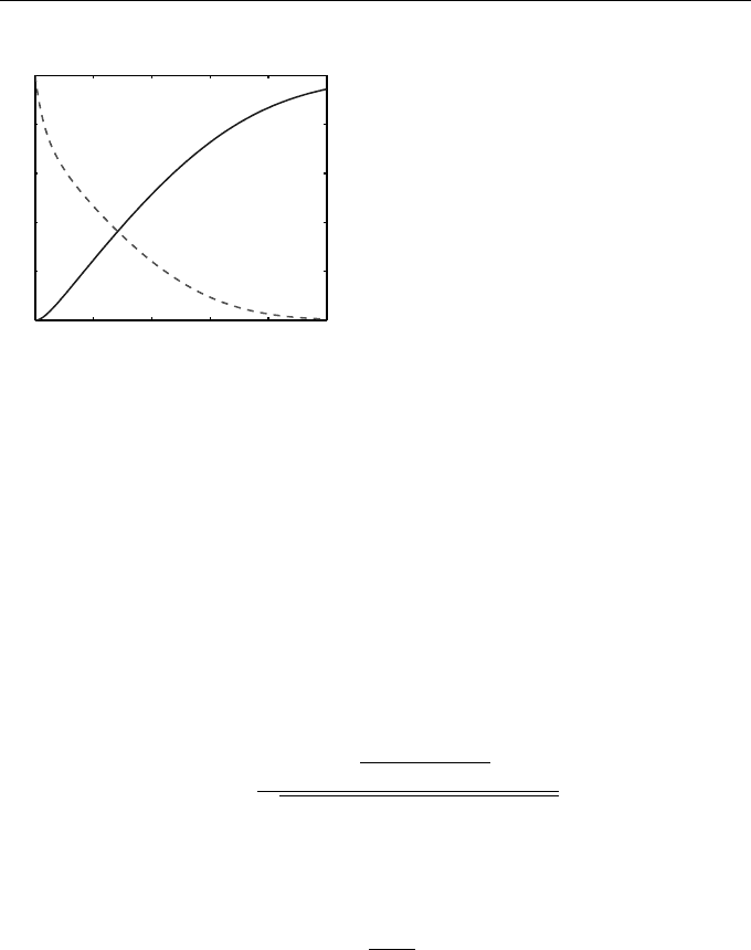
In Figure 1.4 we show how the levels of substrate and product, x

(t) and

(t) respectively, evolve over time. It is clear that the substrate becomes de-

pleted as product is created. Here we took initial conditions of x

(0) = 5×10

−7

(0) = 2 × 10

−7

, x

(0) = x

(0) = 0, with rate constants c

= 10

, c

= 10

−4

= 0.1, based on those in Wilkinson [69] that were also used in Higham [33].

We refer to Alon [1] and Higham [33] for more details about how ODE

models are used in chemistry and biochemistry.

8 1. ODEs—An Introduction

0 10 20 30 40 50

x 10

−7

Concentration

Product

Substrate

Fig. 1.4 Substrate and product con-

centrations from the chemical kinetics

ODE of Example 1.4

Example 1.5 (Fox-Rabbit Pursuit)

Curves of pursuit arise naturally in military and predator-prey scenarios when-

ever there is a moving target. Imagine that a rabbit follows a predeﬁned path,

(r(t), s(t)), in the plane in an attempt to shake oﬀ the attentions of a fox. Sup-

pose further that the fox runs at a speed that is a constant factor k times the

speed of the rabbit, and that the fox chases in such a way that at all time s its

tangent points at the rabbit. Straightforward arguments then show that the

fox’s path (x(t), y(t)) satisﬁes

(t) = R(t) (r(t) − x(t)),

(t) = R(t) (s(t) − y(t)),

where

R(t) =

(t)

+ s

(t)

(r(t) − x(t))

+ (s(t) − y(t))

In the case where the rabbit’s path (r(t), s(t)) is known, this is an ODE system

of the form (1.8) with m = 2 components.

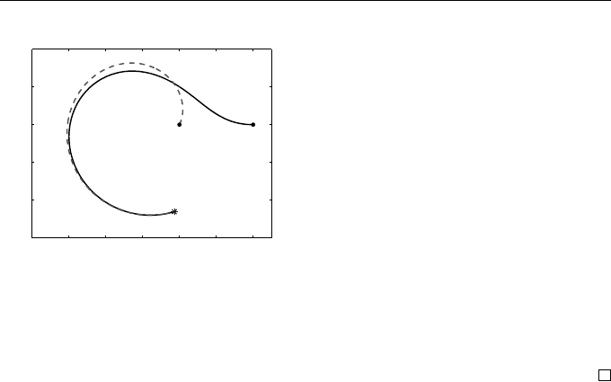
In Figure 1.5 the rabbit follows an outward spiral



r(t)

s(t)



√

1 + t



cos t

sin t



shown as a dashed curve in the x, y plane, with a solid dot marking the initial

location. The fox’s path, found by solving the ODE with a numerical method,

is shown as a solid line. The fox is initially located at x(0) = 3, y(0) = 0

and travels k = 1.1 times as quickly as the rabbit. We solved the ODE up to

t = 5.0710, which is just before the critical time where rabbit and fox meet

(marked by an asterisk). At that point the ODE would be ill deﬁned because

of a division-by-zero error in the deﬁnition of R(t) (and because of a lack of

rabbit!).

1.1 Systems of ODEs 9

−3 −2 −1 0 1 2 3

−3

−2

−1

Fox

Rabbit

Fig. 1.5 Fox-rabbit pursuit curve

from Example 1.5

This example is taken from Higham and Higham [34, Chapter 12], where

further details are available. A comprehensive and very entertaining coverage

of historical developments in the ﬁeld of pursuit curves can be found in Nahin’s

bo ok [58].

Example 1.6 (Zombie Outbreak)

ODEs are often used in epidemiology and population dynamics to describe the

spread of a disease. To illustrate these ideas in an eye-catching science ﬁction

context, Munz et al. [55] imagined a zombie outbreak. At each time t, their

model records the levels of

– humans H(t),

– zombies Z(t),

– removed (‘dead’ zombies) R(t), which may return as zombies.

It is assumed that a zombie may irreversibly convert a human into a zombie. On

the other hand, zombies cannot be killed, but a plucky human may temporarily

send a zombie into the ‘removed’ class. The simplest version of the model takes

the form

(t) = −βH(t)Z(t),

(t) = βH(t)Z(t) + ζR(t) − αH(t)Z(t),

(t) = αH(t)Z(t) − ζR(t).

The (constant, positive) parameters in the model are:

– α, dealing with human–zombie encounters that remove zombies.

– β, dealing with human–zombie encounters that convert humans to zombies.

– ζ, dealing with removed zombies that revert to zombie status.

10 1. ODEs—An Introduction

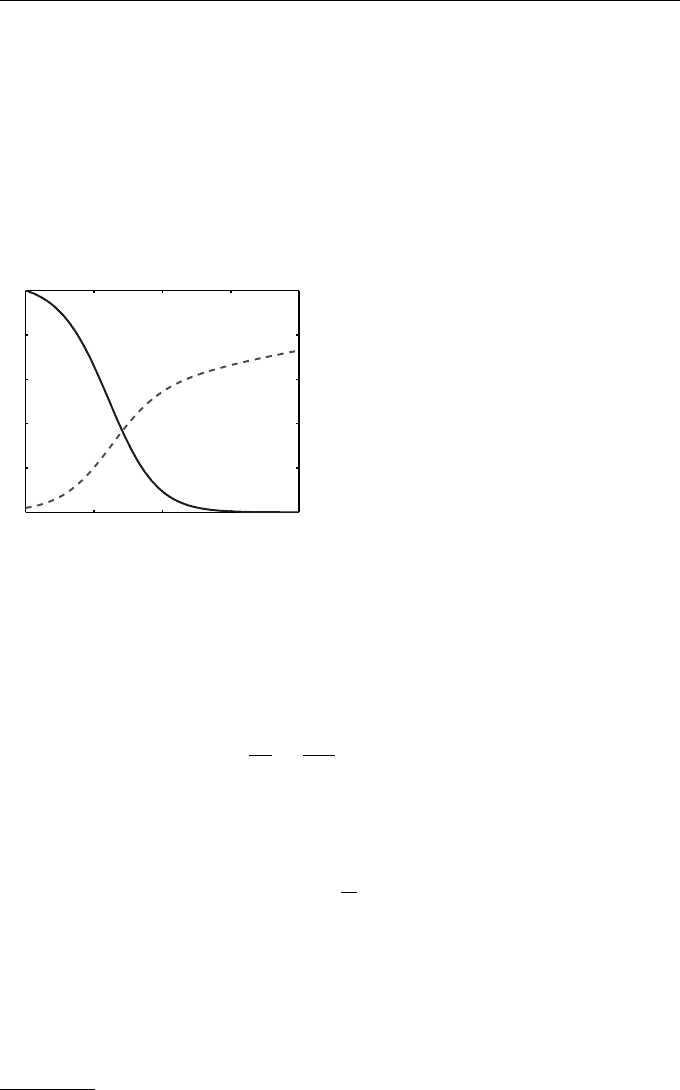
Figure 1.6 shows the case where β = 0.01. α = 0.005 and ζ = 0.02. We

set the initial human population to be H(0) = 500 with Z(0) = 10 zombies.

We have in mind the scenario where a group of zombies from Lenzie, near

Glasgow, attacks the small community of Newport in Fife. The ﬁgure shows

the evolution of the human and zombie levels, and the doomsday outcome of

total zombiﬁcation.

The issue of how to infer the m odel parameters from observed human/zombie

population levels is treated in [7].

0 1 2 3 4

100

200

300

400

500

Humans

Zombies

Fig. 1.6 Human and zombie popula-

tion levels from Example 1.6

Example 1.7 (Method of Lines for Partial Diﬀerential Equations)

The numerical solution of partial diﬀerential equations (PDEs) can lead to

extremely large systems of ODEs. Consider the solution of Fisher’s equation

∂u

∂t

∂

∂x

+ u(1 − u)

deﬁned for 0 < x < 5 and t > 0. The solution u(t, x) also has to satisfy

boundary conditions u(t, 0) = 0 and u(t, 5) = 1, and match given initial data

u(0, x), which we take to be

u(0, x) = e

x/5−1

sin

πx, 0 ≤ x ≤ 5.

This is a simple example of one of the many initial-b oundary-value problems for

equations of reaction-diﬀusion type that occur in chemistry, biology, ecology,

and countless other areas. It can be solved numerically by dividing the interval

0 < x < 5 into 5N subintervals (say) by the points x

= j/N, j = 0 : 5N and

using u

(t) to denote the approximation to u(x

, t) at each of these locations.

After approximating the second derivative in the equation by ﬁnite diﬀerences

For integers m < n, j = m : n is shorthand for j = m, m + 1, m + 2, . . . , n.

1.1 Systems of ODEs 11

(see, for instance, Le veque [47] or Morton and Mayers [54]) we arrive at a

system of 5N − 1 diﬀerential equations, of which a typical equation is

= N

j−1

− 2u

+ u

j+1

) + u

− u

(j = 1 : 5N −1) with end conditions u

(t) = 0, u

(t) = 1 and initial conditions

that specify the values of u

(0):

(0) = e

1−j/5N

sin

10N

π, j = 1 : 5N −1.

By deﬁning the vector function of t

u(t) = [u

(t), u

(t), . . . , u

5N−1

(t)]

and the (5N − 1) × (5N −1) tridiagonal matrix A

A = N







−2 1

1 −2 1

1 −2







(1.11)

we obtain a system of the form

(t) = Au(t) + g(u(t)), t > 0,

where the jth component of g(u) is u

− u

(except for the last component,

5N−1

(u), which has an additional term, N

, due to the non-zero boundary

condition at x = 5) and u(0) = η is the known vector of initial data. The

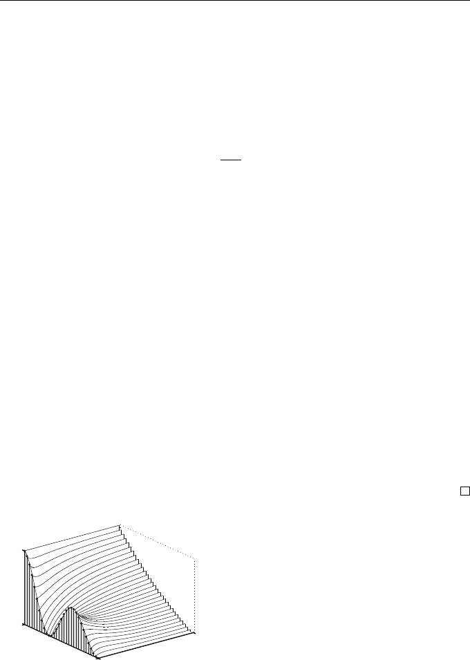
solution with N = 6 is shown in Figure 1.7 for 0 ≤ t ≤ 0.1.

0.1

(t)

Fig. 1.7 Solution for the 29 ODEs

approximating Fisher’s equation with

N = 6. The initial conditions for

the components are indicated by solid

dots (•)

Generally, PDEs involving one spatial variable (x) typically lead to 100–1000

ODEs. With two spatial variables (x and y) these numbe rs become 100

–1000

so the number of ODEs in a system may run to millions.

12 1. ODEs—An Introduction

1.2 Higher Order Diﬀerential Equations

Some mathematical models involve derivatives higher than the ﬁrst. For ex-

ample, Newton’s laws of motion involve acceleration—the second derivative of

position with respect to time. Such higher-order ODEs are automatically con-

tained in the framework of systems of ﬁrst-order ODEs. We ﬁrst illustrate the

idea with an example.

Example 1.8 (Van der Pol Oscillator)

For the second-order IVP

(t) + 10(1 − x

(t))x

(t) + x(t) = sin πt,

x(t

) = η

, x

) = η

we deﬁne u = x, v = x

so that

(t) = v(t),

(t) = −10(1 − u

(t))v(t) − u(t) + sin πt,

with initial conditions u(t

) = η

and v(t

) = η

. These equations are now in

the form (1.7), so that we may again write them as (1.8), where

x(t) =



u(t)

v(t)



, f(t, x(t)) =



v(t)

−10



1 − u

(t)



v(t) − u(t) + sin πt



The solution of the unforced equation, where the term sin πt is dropped, for

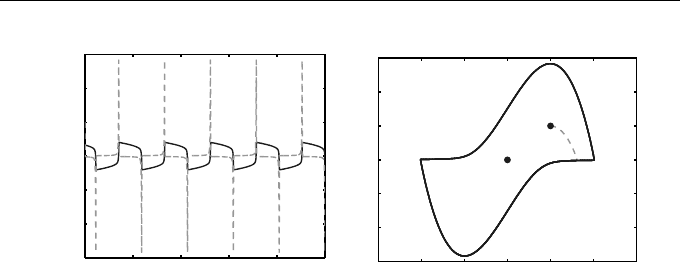
the initial condition u(0) = 1, v(0) = 5 is shown in Figure 1.8 for 0 ≤ t ≤ 100.

After a short initial phase (0 ≤ t ≤ 0.33—shown as a broken curve emanating

from P) the solution approaches a periodic motion; the limiting closed curve

is known as a limit cycle. In the ﬁgure on the left the solution v(t) ≡ x

(t) is

shown as a broken curve and appears as a sequence of spikes.

It is straightforward to extend the s ec ond-order example in Example 1.8 to

a diﬀerential equation of order m:

(m)

(t) = f



t, x(t), x

(t), . . . , x

(m−1)

(t)



. (1.12)

New dependent variables may be introduced for the function x(t) and each of

its ﬁrst (m − 1) derivatives:

(t) = x(t),

(t) = x

(t),

(t) = x

(m−1)

(t).

1.2 Higher Order Diﬀerential Equations 13

0 20 40 60 80 100

−15

−10

−5

u(t), v(t)

−3 −2 −1 0 1 2 3

−15

−10

−5

Fig. 1.8 Solution for the ODEs representing the unforced Van der Pol equa-

tion of Example 1.8. On the left, u(t) ≡ x(t) (solid curve) and v(t) ≡ x

(t)

(broken curve) are shown as functions of t. The phase portrait is drawn on the

right, where P marks the initial point

There are obvious relationships between the ﬁrst (m − 1) such functions:

(t) = x

(t),

(t) = x

(t),

m−1

(t) = x

(t).

These, together with the diﬀerential equation, which has become,

(t) = f (t, x

(t), x

(t), . . . , x

(t)),

give a total of m ODEs for the components of the m-dimensional vector function

x = [x

, x

, . . . , x

]

. The corresponding IVP for x(t) has values speciﬁed for

the function itself as well as its ﬁrst (m − 1) derivatives at the initial time

t = t

, and these give directly the initial conditions for the m components of

x(t

). We therefore have an IVP of the form (1.8), where

f(t, x(t)) =







(t)

f(t, x

(t), x

(t), . . . , x

(t))







, η =







x(0)

(0)

(m−2)

(0)

(m−1)

(0)







The general principle in this book is that numerical methods will be constructed

and analysed, in the ﬁrst instance, for approximating the solutions of IVPs for

scalar problems of the form given in (1.6), after which we will discuss how the

same methods apply to problems in the vector form (1.8).

14 1. ODEs—An Introduction

1.3 Some Model Problems

One of our strategies in assessing numerical methods is to apply them to very

simple problems to gain understanding of their behaviour and then attempt to

translate this understanding to more realistic scenarios.

Examples of simple model ODEs are:

1. x

(t) = λx(t), x(0) = 1, λ ∈ <; usually λ < 0 so that x(t) → 0 as t → ∞.

2. x

(t) = ix(t), x(0) = 1 (i =

√

−1) modelling oscillatory motion (see Exer-

cise 1.6).

3. x

(t) = −100x(t) + 100e

−t

, x(0) = 2. The exact solution is x(t) = e

−t

−100t

, which combines two decaying terms, one of which is very rapid and

one that decays more slowly. Hence, there are two distinct time scales in

this solution.

4. x

(t) = 1, x(0) = 0.

5. x

(t) = 0, x(0) = 0.

The last two, in particular, are trivial, but of course, a numerical method, if

it is to be useful, must work well on such simple examples—if methods cannot

reproduce the solutions to these problems then they are deemed to be un-

suitable for solving any IVPs. Through use of simple ODEs we can highlight

deﬁciencies; and the simpler the ODE, the simpler the analysis is.

Example 1.9 (A Cooling Cup of Coﬀee)

Although linear ODEs such as 1–5 above are useful for testing numerical meth-

ods, they may also arise as mathematical models. For example, suppose that

a cup of boiling coﬀee is prepared at time t = 0 and cools according to New-

ton’s law of cooling: the rate of change of te mperature is prop ortional to the

diﬀerence in temperature between the coﬀ ee and the surrounding room (see,

for instance, Chapter 12 of Fulford et al. [20]). Suppose that u(t) represents

the coﬀee temperature (in degrees Celsius) after t hours. This leads to the

diﬀerential equation

(t) = −α(u(t) − v),

where α is known as the rate constant (which will be taken to be α = 8

◦

C h

−1

)

and v represents room temperature. We consider a number of scenarios (see Fig-

ure 1.9).

Recall that the function A e

−λt

(λ ∈ R) decays to half its initial value (A at

t = 0) in a time t = (log 2)/λ ≈ 0.7/λ, commonly referred to as its half-life. The

larger the rate constant λ is, the more quickly it decays.

1.3 Some Model Problems 15

1. Room temperature is a constant v = 20

◦

C. We then have a scalar IVP

(t) = −8(u(t) − 20), u(0) = 100. (1.13)

This has solution u(t) = 80e

−8t

+ 20.

2. The room is also cooling ac cording to Newton’s law from an initial temper-

ature of 20

◦

C with a rate constant 1/8 and exterior temperature of 5

◦

With v(t) denoting room temperature, we have the following system of two

ODEs

(t) = −8(u(t) − v(t)), u(0) = 100,

(t) = −(v(t) − 5)/8, v(0) = 20.

(1.14)

The second of these ODEs may be solved to give

v(t) = 15e

−t/8

+ 5,

which can be used to give a scalar IVP for u:

(t) = −8(u(t) − 15e

−t/8

− 5), u(0) = 100. (1.15)

It follows that u(t) =

1675

−8t

320

−t/8

+ 5 (see Exercise 1.13).

3. There is a third situation where the coﬀee container is well insulated and

the room is not. We may model this by the IVP

(t) = −

(u(t) − 5 + 5025e

−8t

), u(0) = 100, (1.16)

so that it has the same solution as (1.15). Although the two problems have

the same solution, numerical methods applied to the two problems will

generally behave diﬀerently, and this will be explored in due course (see

Examples 6.1 and 6.2).

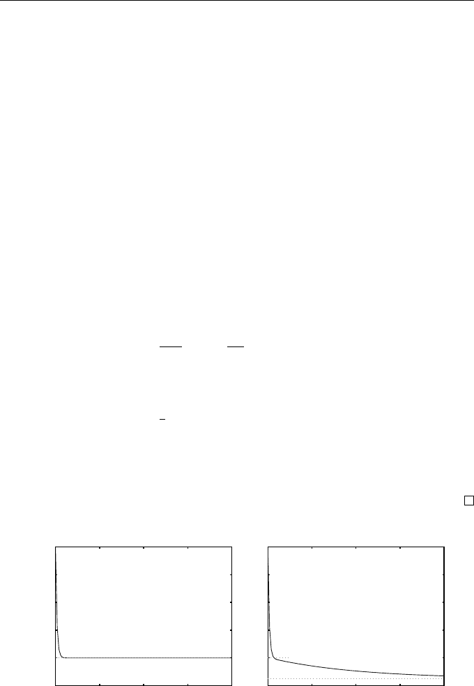
0 4 8 12 16

100

u(t)

0 4 8 12 16

100

u(t)

Fig. 1.9 The solution of (1.13) (left) and (1.14)–(1.16) (right)