Griffiths D.F., Higham D.J. Numerical Methods for Ordinary Differential Equations: Initial Value Problems
Подождите немного. Документ загружается.

26 2. Euler’s Method
that the numerical solution should approach the exact s olution, i.e. the size of
the GE
|e
n
| ≡ |x(t
n
) − x
n
|
at t = t
0
+ nh should also decrease. This is intuitively reasonable; as we put
in more computational effort, we should obtain a more accurate solution. The
situation is, however, a little more subtle than is immediately apparent. If we
were to consistently compare, say, the fourth terms in the sequences {x(t
n
)}
and {x
n
} computed with h = 0.5, 0.25, and 0.125, then we would compute the
error at t
4
= t
0
+ 2.0, t
0
+ 1.0 and t
0
+ 0.5, respectively. That is, we would be
comparing errors at different times when different values of h were employed.
Even more worryingly, as h → 0, t
4
= t
0
+ 4h → t
0
, and we would eventually
be comparing x
4
with x(t
0
) = η—the initial condition. What must be done is
to compare the exact solution of the IVP and the numerical solution at a fixed
time t = t
∗
, say, within the interval of integration. For this, the relevant value
of the index n is calculated from t
n
= t
0
+ nh = t
∗
, or n = (t
∗
−t
0
)/h, so that
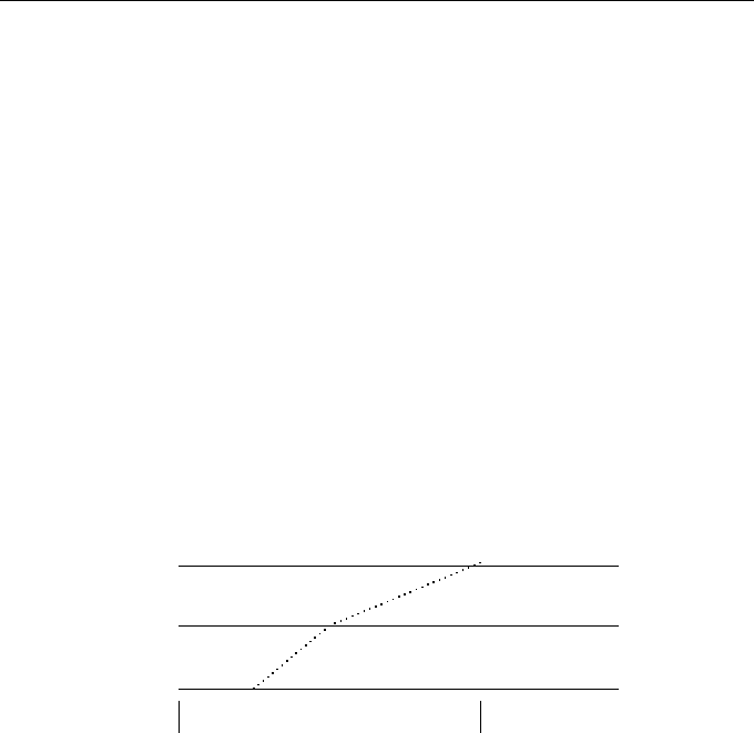
n → ∞ as h → 0. The situation is illustrated in Figure 2.4.
h = 0.125 : r r r r r r r r r r r r r r r r r r r r r
t
0
t
2
t
4
t
16
h = 0.25 : r r r r r r r r r r r
t
0
t
1
t
2
t
3
t
4
t
8
h = 0.5 :
r r r r r r
t
0
t
1
t
2
t
3
t
4
6
t = 0
6
t = 2
Fig. 2.4 The grids associated with grid sizes h = 0.5, 0.25, and 0.125
Some results from Euler’s method were analysed in Section 2.1.1 and it ap-
peared that the GE was proportional to h: e
n
∝ h when nh = 0.9, suggesting
that the GEat t
∗
= 0.9 could be made arbitrarily small by choosing a corre-
spondingly small step size h. That is, we could, were we prepared to take a
sufficient number of small steps, obtain an approximation that was as accurate
as we pleased. This suggests that the Euler’s method is convergent.
Definition 2.3
A numerical method is said to converge to the solution x(t) of a given IVP at
t = t
∗
if the GE e
n
= x(t
n
) − x
n
at t
n
= t
∗
satisfies
|e
n
| → 0 (2.12)

2.4 Analysing the Method 27
as h → 0. It converges at a pth-order rate if e
n
= O(h
p
) for some p > 0.
3
We will take the view that numerical methods are of no value unless they
are convergent—so any desired accuracy can be guaranteed by taking h to be
sufficiently small.
It may be proved that Euler’s method converges for IVPs of the form given
by Equation (2.1) whenever it has a unique solution for t
0
≤ t ≤ t
f
. However,
the proof (see Hairer et al. [28] or Braun [5]) is rather technical owing to the
fact that it has to cope with a general nonlinear ODE. We shall therefore
be less ambitious and provide a proof only for a linear constant-coefficient
case; the conclusions we draw will be relevant to more general situations. In
particular, the result will indicate how the local errors committed at each step
by truncating a Taylor series accumulate to produce the GE.
Theorem 2.4
Euler’s method applied to the IVP
x
0
(t) =λx(t) + g(t), 0 < t ≤ t
f
,
x(0) =1,
where λ ∈ C and g is a continuously differentiable function, converges and the
GE at any t ∈ [0, t
f
] is O(h).
Proof
Euler’s method for this IVP gives
x
n+1
= x
n
+ λhx
n
+ hg(t
n
) = (1 + λh)x
n
+ hg(t
n
) (2.13)
while, from the Taylor series expansion (2.5) of the exact solution,
x(t
n+1
) = x(t
n
) + hx
0
(t
n
) + R
1
(t
n
),
= x(t
n
) + h
λx(t
n
) + g(t
n
)
+ R
1
(t
n
). (2.14)
By subtracting (2.13) from (2.14) we find that the GE e
n
= x(t
n
) − x
n
satisfies
the difference equation
e
n+1
= (1 + hλ)e
n
+ T
n+1
, (2.15)
where we have written T
n+1
instead of R
1
(t
n
) to simplify the notation. Fur-
thermore, since x
0
= x(t
0
) = η, we have e
0
= 0. Equation (2.15) dictates how
3
By convention we refer to the largest such value of p as the “order of the method.”

28 2. Euler’s Method
the GE at the next step (e
n+1
) combines the LTE committed at the current
step (T
n+1
) with the GE inherited from earlier steps (e
n
). A similar equation
holds for more general ODEs although λ would have to be allowed to vary from
step to step.
Substituting n = 0, 1, 2 into (2.15) we find, using e
0
= 0,
e
1
= T
1
,
e
2
= (1 + hλ)e
1
+ T
2
= (1 + hλ)T
1
+ T
2
,
e
3
= (1 + hλ)e
2
+ T
3
= (1 + hλ)
2
T
1
+ (1 + hλ)T
2
+ T
3
,
which suggests the general formula
4
e
n
= (1 + hλ)
n−1
T
1
+ (1 + hλ)
n−2
T
2
+ ··· + T
n
=
n
X
j=1
(1 + hλ)
n−j
T
j
. (2.16)
All that remains is to find an upper bound for the right-hand side. First, using
Exercise 2.8 (with x = |λ|),
|1 + hλ| ≤ 1 + h|λ| ≤ e
h|λ|
and so
|1 + hλ|
n−j
≤ e
(n−j)h|λ|
= e
|λ|t
n−j
≤ e
|λ|,t
f
since (n − j)h = t
n−j
≤ t
f
for nh ≤ t
f
and 0 < j ≤ n.
Second, since |T
j
| ≤ C h
2
for some constant C (independent of h or j), each
term in the summation on the right of (2.16) is bounded by h
2
C e
|λ|t
f
and so
|e
n
| ≤ nh
2
C e
|λ|t
f
= ht
f
C e
|λ|t
f
(using nh = t
f
). Thus, so long as t
f
is finite, e
n
= O(h) and we have proved
that Euler’s method converges at a first-order rate.
The proof makes it clear that the contribution of the LTE T
j
at time t = t
j
to the approximation of x
n
at time t = t
n
is (1 + hλ)
n−j
T
j
, with 1 + hλ > −1.
The LTE is amplified if λ is real and positive, and diminished if λ is real
and negative. The most important observation, however, is that an LTE T
n
=
O(h
p+1
) of order (p + 1) leads to a GE e
n
= O(h
p
) of order p; the cumulative
effect of introducing a truncation error at each step is to lose one power of h.
4
This can be proved to be correct either by the process described in Exercise 2.9
or by induction.

2.5 Application to Systems 29
2.5 Application to Systems
We shall illustrate by an example how Euler’s method applies to systems of
ODEs.
Example 2.5
Use Euler’s me thod to compute an approximate solution at t = 0.2 of the IVP
x
00
(t) + x(t) = t, t > 0, with x(0) = 1 and x
0
(0) = 2. Use a s tep length h = 0.1.
In order to convert the second-order equation to a system, let u = x and v = x
0
,
so v
0
= u
00
= x
00
= −u + t. This gives the system
u
0
(t) = v(t)
v
0
(t) = t − u(t)
(2.17)
on the interval t > 0 with initial conditions u(0) = 1, v(0) = 2. By Taylor series,
u(t + h) = u(t) + hu
0
(t) + O(h
2
),
v(t + h) = v(t) + hv
0
(t) + O(h
2
).
Neglecting the remainder terms gives Euler’s method for the s ystem (2.17):
t
n+1
= t
n
+ h,
u
n+1
= u
n
+ hu
0
n
, u
0
n+1
= v
n+1
,
v
n+1
= v
n
+ hv
0
n
, v
0
n+1
= t
n+1
− u
n+1
.
Note that both u
n+1
and v
n+1
must generally be calculated before calculat-
ing the derivative approximations u
0
n+1
and v
0
n+1
. The starting conditions are
u
0
= 1, v
0
= 2 at t = t
0
= 0 and the given differential equations lead to
u
0
0
= v
0
= 2 and v
0
0
= t
0
− u
0
= −1. Applying the above recurrence relations
first with n = 0 and then n = 1 gives
n = 0 : t
1
= 0.1, n = 1 : t
2
= 0.2,
u
1
= u
0
+ 0.1u
0
0
= 1.2, u
2
= 1.39,
v
1
= v
0
+ 0.1v
0
0
= 1.9, v
2
= 1.79,
u
0
1
= 1.9, u
0
2
= 1.79,
v
0
1
= t
1
− u
1
= −1.1, v
0
2
= t
2
− u
2
= −1.19.
The computations proceed in a similar fashion until the required end time is
reached.

30 2. Euler’s Method
EXERCISES
2.1.
?
Use Euler’s method with h = 0.2 to show that the solution of the
IVP x
0
(t) = t
2
−x(t)
2
, t > 0, with x(0) = 1 is approximately x(0.4) ≈
0.68.
Show that this estimate changes to x(0.4) ≈ 0.708 if the calculation
is repeated with h = 0.1.
2.2.
??
Obtain the recurrence relation that enables x
n+1
to be calculated
from x
n
when Euler’s method is applied to the IVP x
0
(t) = λx(t),
x(0) = 1 with λ = −10. In each of the cases h = 1/6 and h = 1/12
(a) calculate x
1
, x
2
and x
3
,
(b) plot the points (t
0
, x
0
), (t
1
, x
1
), (t
2
, x
2
), and (t
3
, x
3
) and compare
with a sketch of the exact solution x(t) = e
λt
.
Comment on your results. What is the largest value of h that can
be used when λ = −10 to ensure that x
n
> 0 for all n = 1, 2, 3, . . .?
2.3.
??
Apply Euler’s method to the IVP
x
0
(t) = 1 + t − x(t), t > 0
x(0) = 0
.
Calculate x
1
, x
2
, . . . and deduce an expression for x
n
in terms of
t
n
= nh and thereby guess the exact solution of the IVP. Use the
expression (2.6) to calculate the LTE and then appeal to the proof
of Theorem 2.4 to explain why x
n
= x(t
n
).
2.4.
?
Derive Euler’s method for the first-order system
u
0
(t) = −2u(t) + v(t)
v
0
(t) = −u(t) − 2v(t)
with initial conditions u(0) = 1, v(0) = 0. Use h = 0.1 to compute
approximate values for u(0.2) and v(0.2).
2.5.
?
Rewrite the IVP
x
00
(t) + x(t)x
0
(t) + 4x(t) = t
2
, t > 0,
x(0) = 0, x
0
(0) = 1,
as a first-order system and use Euler’s metho d with h = 0.1 to
estimate x(0.2) and x
0
(0.2).
2.6.
?
Derive Euler’s method for the first-order systems obtained in Exer-
cise 1.5 (b) and (c).

Exercises 31
2.7.
???
This question concerns approximations to the IVP
x
00
(t) + 3x
0
(t) + 2x(t) = t
2
, t > 0,
x(0) = 1, x
0
(0) = 0.
(2.18)
(a) Write the above initial value problem as a first-order system
and hence derive Euler’s method for computing approximations
to x(t
n+1
) and x
0
(t
n+1
) in terms of approximations to x(t
n
) and
x
0
(t
n
).
(b) By eliminating y, show that the system
x
0
(t) = y(t) − 2x(t)
y
0
(t) = t
2
− y(t)
has the same solution x(t) as the IVP (2.18) provided that
x(0) = 1, and that y(0) is suitably chosen. What is the ap-
propriate value of y(0)?
(c) Apply Euler’s method to the system in part (b) and give for-
mulae for computing approximations to x(t
n+1
) and y(t
n+1
) in
terms of approximations to x(t
n
) and y(t
n
).
(d) Show that the approximations to x(t
2
) produced by the methods
in (a) and (c) are identical provided both methods use the same
value of h.
2.8.
??
Prove that e
x
≥ 1 + x for all x ≥ 0. [Hint: use the fact that e
t
≥ 1
for all t ≥ 0 and integrate both sides over the interval 0 ≤ t ≤ x
(where x ≥ 0).]
2.9.
??
Replace n by j −1 in the recurrence relation (2.15) and divide both
sides by (1 + λh)
j
to obtain
e
j
(1 + λh)
j
−
e
j−1
(1 + λh)
j−1
=
T
j
(1 + λh)
j
.
By summing both sides from j = 1 to j = n, show that the result
simplifies to give Equation (2.16).
3
The Taylor Series Method
3.1 Introduction
Euler’s method was introduced in Chapter 2 by truncating the O(h
2
) terms
in the Taylor series of x(t
h
+ h) about the point t = t
n
. The accuracy of the
approximations generated by the method could be controlled by adjusting the
step size h—a strategy that is not always practical, since one may need an
inordinate number of steps for high accuracy. For instance, around 1 million
steps are necessary to solve the IVP of Example 2.1 to an accuracy of about
10
−6
for 0 ≤ t ≤ 1.
An alternative is to use a m ore sophisticated recurrence relation at each
step in order to achieve greater accuracy (for the same value of h) or a similar
level of accuracy with a larger value of h (and, therefore, fewer steps).
There are many ways of attaining this goal. In this chapter we inve stigate
the possibility of improving the efficiency by including further terms in the
Taylor series. Other m eans will be developed in succeeding chapters.
We shall again be concerned with the solution of an IVP of the form
x
0
(t) = f (t, x), t > t
0
x(t
0
) = η
(3.1)
over the interval, t ∈ [t
0
, t
f
]. We describe a second-order method before treating
the case of general order p.
Springer Undergraduate Mathematics Series, DOI 10.1007/978-0-85729-148-6_3,
© Springer-Verlag London Limited 2010
D.F. Griffiths, D.J. Higham, Numerical Methods for Ordinary Differential Equations,

34 3. The Taylor Series Method
3.2 An Order-Two Method: TS(2)
As discussed in Appendix B, the second-order Taylor series expansion
x(t + h) = x(t) + hx
0
(t) +
1
2!
h
2
x
00
(t) + R
2
(t)
has remainder term R
2
(t) = O(h
3
). Setting t = t
n
we obtain (since t
n+1
=
t
n
+ h)
x(t
n+1
) = x(t
n
) + hx
0
(t
n
) +
1
2!
h
2
x
00
(t
n
) + O(h
3
).
Neglecting the remainder term on the grounds that it is small leads to the
formula
x
n+1
= x
n
+ hx
0
n
+
1
2
h
2
x
00
n
, (3.2)
in which x
n
, x
0
n
, and x
00
n
denote approximations to x(t
n
), x
0
(t
n
), and x
00
(t
n
)
respectively. We shall refer to this as the TS(2) method (some authors call it
the three-term TS method—in our naming regime, Euler’s method becomes
TS(1)). As in Chapter 2, the value of x
0
n
can be computed from the IVP (3.1):
x
0
n
= f(t
n
, x
n
).
For x
00
n
we need to differentiate both sides of the ODE, as illustrated on the fol-
lowing example (which was previously used in Example 2.1 for Euler’s method).
Example 3.1
Apply the TS(2) method (3.2) to solve the IVP
x
0
(t) = (1 − 2t)x(t), t > 0
x(0) = 1
(3.3)
using h = 0.3 and h = 0.15 and compare the accuracy at t = 1.2 with that of
Euler’s method, given that the exact solution is x(t) = exp[
1
4
− (t −
1
2
)
2
].
In order to apply the formula (3.2) we must express x
00
(t) in terms of x(t) and
t (it could also involve x
0
(t), but this can be substituted for from the ODE):
with the chain rule we find (the general case is dealt with in Exercise 3.9)
x
00
(t) =
d
dt
[(1 − 2t)x(t)] = −2x(t) + (1 − 2t)x
0
(t)
= [(1 − 2t)
2
− 2]x(t),
and so the TS(2) method is given by
x
n+1
= x
n
+ h(1 − 2t
n
)x
n
+
1
2
h
2
[(1 − 2t
n
)
2
− 2]x
n
, n = 0, 1, . . . ,
3.2 An Order-Two Metho d: TS(2) 35
where t
n
= nh and x
0
= 1. For the purposes of hand calculation it can be
preferable to use (3.2) and arrange the results as shown below:
n = 0 : t
0
= 0 , n = 1 : t
1
= t
0
+ h = 0.3,
x
0
= 1, x
1
= x
0
+ hx
0
0
+
1
2
h
2
x
00
0
= 1.2550,
x
0
0
= 1, x
0
1
= (1 − 2t
1
)x
1
= 0.5020,
x
00
0
= −1, x
00
1
= [(1 − 2t
1
)
2
− 2]x
1
= −2.3092,
with a similar layout for n = 2, 3, . . ..
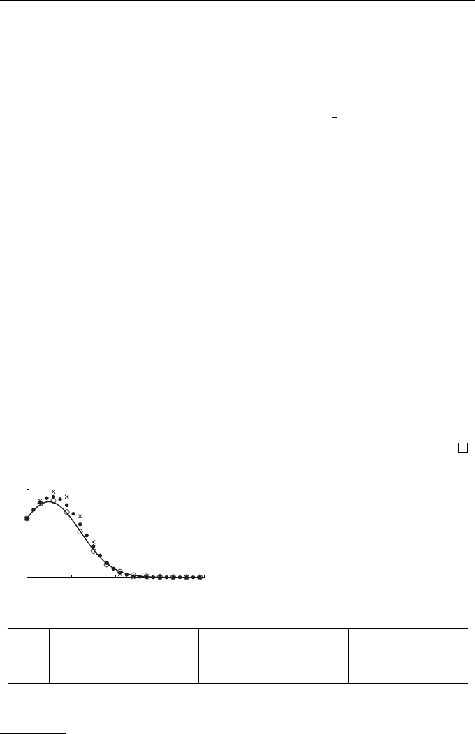
In Figure 3.1 the computations are extended to the interval 0 ≤ t ≤ 4 and
the numerical values with associated GEs at t = 1.2 are tabulated in Table 3.1.
We observed in Example 2.1 that the GE in Euler’s me thod was halved by
halving h, reflec ting the relationship e
n
∝ h. However, from Table 3.1, we see
that the error for the TS(2) method is reduced by a factor of roughly 4 as h is
halved (0.0031 ≈ 0.0118/4), suggesting that the GE e
n
∝ h
2
.
We deduce from Table 3.1 that, at t = 1.2,
1
GE for Euler’s method ≈ −0.77h
GE for TS(2) method ≈ 0.14h
2
.
These results suggest that, to achieve an accuracy of 0.01, the step size in
Euler’s method would have to satisfy 0.77h = 0.01, from which h ≈ 0.013 and
we would need about 1.2/0.013 ≈ 92 steps to integrate to t = 1.2. What are
the corresponding values for TS(2)? (Answer: h ≈ 0.27 and five steps). This
illustrates the huge potential advantages of using a higher order method.
0 1 2 3 4
0
0.5
1
1.5
t
n
x
n
Fig. 3.1 Numerical solutions for
Example 3.1
× : Euler’s method, h = 0.3,
• : Euler’s method, h = 0.15,
◦ : TS(2) method, h = 0.15.
Solutions at t = 1.2 GEs at t = 1.2
h Euler: TS(1) TS(2) Euler: TS(1) TS(2) GE for TS(2)/h
2
0.30 1.0402 0.7748 −0.2535 0.0118 0.131
0.15 0.9014 0.7836 −0.1148 0.0031 0.138
Table 3.1 Numerical solutions and global errors at t = 1.2 for Example 3.1.
The exact solution is x(1.2) = e
−0.24
= 0.7866.
1
These relations were deduced from the assertions e
n
= C
1
h for Euler and e
n
=
C
2
h
2
for TS(2) and choosing the constants C
1
, C
2
so as to match the data in Table 3.1
for h = 0.15.