Gubbins D., Herrero-Bervera E. Encyclopedia of Geomagnetism and Paleomagnetism

Подождите немного. Документ загружается.

Langel, R.A., and Estes, R.H., 1982. A geomagnetic field spectrum.

Geophysical Research Letters , 9 : 250– 253.

Langel, R.A., and Hinze, W.J., 1998. The Magnetic Field of the

Earth ’s Lithosphere. Cambridge: Cambridge University Press.

Lowes, F.J., 1974. Spatial power spectrum of the main geomagnetic

field, and extrapolation to the core. Geophysical Journal of Royal

Astronomical Society, 36: 717–730.

Purucker, M., Langel, R., Rajaram, M., and Raymond, C., 1998.

Global magnetization models with a priori information. Journal

of Geophysical Research, 103 : 2563– 2584.

Sabaka, T.J., Olsen, N., and Langel, R.A., 2002. A comprehensive

model of the quiet-time, near-Earth magnetic field: phase 3. Geo-

physical Journ al International , 151:32– 68.

Sabaka, T.J., Olsen, N., and Purucker, M., 2004, Extending compre-

hensive models of the Earth ’s magnetic field with Oersted and

CHAMP data. Geophysical Journal International , 159: 521– 547.

Taylor, P., and Purucker, M., 2000. Robert A. Langel III (1937– 2000).

EOS. Transactions of the American Geophysical Union, 81(1 5) : 1 59 .

Cross- refere nces

Harmonics, Spherical

IAGA, International Association of Geomagnetism and Aerono my

Magsat

LAPLACE’S EQUATION, UNIQUENESS

OF SOLUTIONS

Potential theory lies at the heart of geomagnetic field analysis. In

regions where no currents flow the magnetic field is the gradient of

a potential that satisfies Laplace ’s equation:

B ¼rV (Eq. 1)

V ¼ 0 (Eq. 2)

We can find the geomagnetic potential V everywhere in the source-free

region by solving Eq. (2) subject to appropriate boundary conditions.

Equation (1) means that we are dealing with a single scalar, the geo-

magnetic potential, and Eq. (2) means that we only have to know that

scalar on surfaces rather than throughout the entire region. This

reduces the number of measurements enormously. I shall discuss here

two idealized situations appropriate to geomagnetism and paleomagnet-

ism: measurements on a plane in Cartesian coordinate s (x, y, z) with z

down, continued periodically in x and y, appropriate for a small survey,

and measurements on a spherical surface r ¼ a in spherical coordinates

ð r ; y; fÞ , where a is Earth ’ s radius. Simple generalizations are possible

to more complex surfaces.

It is well known that solutions of Laplace ’s equation within a volume

O are unique when V is prescribed on the bounding surface ] O, the

so-called Dirichlet conditions. This is of no use to us because we cannot

measure the geomagnetic potential directly. We can, however, measure

the component of magnetic field normal to the surface, which also

guarantees uniqueness (the so-called Neumann conditions). Thus mea-

surement of a single component of magnetic field on a surface can be

used to reconstruct the magnetic field throughout the current-free region,

provided the sources are entirely inside or outside the measurement

surface. When both internal and external sources are present two com-

ponents need to be measured on a single surface, when it is also possible

to separate the parts (see Internal external field separation ). Here I

shall focus on the case of purely internal sources.

Components other than the vertical also provide uniqueness.

As illustration consider the general solutio n of Laplace’ s equation in

Cartesian coordinates:

V ðx ; y; zÞ¼

k ;l ;m

expð mz Þ cos ð kx þ‘ y þ a

k ;‘

Þ; (Eq. 3)

where m ¼

ﬃﬃﬃﬃﬃﬃﬃﬃﬃﬃﬃﬃﬃﬃﬃ

þ‘

is positive to ensure a finite solution as z !1

and the f a

k ;‘

g are phase factors. If B

¼ ] V = ] z is known on z ¼ 0we

can differentiate Eq. (3) with respect to z, set z ¼ 0, and determine the

arbitrary coefficients fC

k ;‘

; a

k ;‘

g from the usual rules for Fourier ser-

ies. This is the case of Neumann boundary conditions. Of course, solu-

tions of Eq. (3) are periodic in x and y with periods 2p = k and 2p = l ,

respectively. B

and B

, however, do not give unique solutions. Differ-

entiating Eq. (3) with respect to x and putting z ¼ 0, for example,

allows determination of all the Fourier coefficients except those with

k ¼ 0. The ambiguity in the solution takes the form V

ð y ; z Þ¼

exp ð lz Þ cos ð ly þ a

Þ: Similarly, measurement only of B

leaves an ambiguity independent of y. Knowing B

and B

overdeter-

mines the problem.

The spherical case is slightly different. B

( Z in conventional geo-

magnetic notation) provides Neumann boundary conditions and so will

give a unique solution. B

(east) allows an axisymmetric ambiguity

similar to that for the cartesian B

and B

cases. Surprisingly,  B

(north) gives a unique solution; the condition that V be finite at the poles

provides the necessary constraint to remove the arbitrary parts of

the solution. Proof involves the general solution of Laplace ’s equation

as a spherical harmonic expansion (see Main field modeling ) in similar

fashion to the use of the Fourier series solution in the cartesian case

(see Magnetic anomalies, modeling). More elegant formal proofs of

these standard results making use of Green ’s theorem are to be found

in texts on potential theory (e.g., Kellogg (1953)).

Formal mathematical results dictate the type of measurements we

must make in order to obtain meaningful estimates of the geomagnetic

field in the region around the observation surface. Clearly in the real

situation other complicat ions arise from finite resolution and errors,

but with a uniqueness theorem we can at least be confident that the

derived field will converge toward the correct field as the data are

improved; for this to happen we must measure the right components

of magnetic field, but this is not always possible. Instrumentation has

changed over the years, dictating changes in the type of measurement

available. Ta b l e L 1 gives a summary of the bias in available datasets.

Backus (1970) addressed the problem of uniqueness when only F

is known on the surface. He showed that, for certain magnetic field

configuratio ns, there exist pairs of magnetic fields B

and B

, which

satisfy rB ¼ 0 and r B ¼ 0 outside ] O and such that

j B

j¼jB

j everywhere on ] O , but jB

j6¼jB

j elsewhere. This result

led to the decision to make vector measurements on the MAGSAT

satellite. In practice B obtained from intensity measurements alone

can differ by 1000 nT from the correct vector measurements. The dif-

ference takes the form of a spheri cal harmonic series with terms domi-

nated by l ¼ m, now called the Backus ambiguity or series. Additional

information does provide uniqueness (e.g., locating the dip equator

(Khokhlov et al., 1997)).

Backus (1968, 1970) gives details of the proof in both two and

three dimensions. The 2D proof uses complex variable theory and is

particularly simple and illuminating. We use the complex potential

w(z), where z ¼ x þ iy. The field is given by the real and imaginary

parts of dw/dz, and jdw=dzj is known on the bounding circle. Focus

attention on

zðzÞ¼ilogdw=dz ¼xþi ¼argjdw=dzjþilogjdw=dzj: (Eq. 4)

Both x and  satisfy Laplace’s equation as the real and imaginary parts of

an analytic function, except where dw=dz ¼ 0. When such singularities

exist, taking a circuit enclosing the source region gives an increase of

2p in the argument of the logarithm. This defines the ambiguity. The

number of singularities determines the number of different solutions; sin-

gularities exist if the field has more than two dip poles on the surface.

Paleomagnetic and older geomagnetic data sets are dominated

by directional measurements. Early models made the reasonable but

466 LAPLACE’S EQUATION, UNIQUENESS OF SOLUTIONS

unproven assumption that direction determined the magnetic field up to

a single multiplicative factor. Proctor and Gubbins (1990) found a result

in 2D using Backus’ method above, focussing instead on the potential

zðzÞ¼logdw=dz ¼ logjdw=dzjþiargjdw=dzj: (Eq. 5)

The above argument then leads to a general solution with one arbitrary

multiplicative constant plus n  1 additional arbitrary constants, where

2n is the number of dip poles.

As with the intensity problem, extension of the 2D proof into 3D

is not straightforward. Proctor and Gubbins (1990) conjectured a

similar result in 3D and provided an axisymmetric example. They also

gave a practical recipe for determining the ambiguity using standard

methods of inverse theory. The problem is homogeneous in the sense

that, if B

and B

are fields derived from harmonic potentials and

are parallel on ]O, then any linear combination of the form

þ a

is also a solution. Thus, having found one solution, B

say, a linear error analysis around B

will yield a direction in solution

space along B

 B

that defines an annihilator for the problem.

Homogeneity then guarantees that this linearized analysis will be valid

globally. Application of this procedure to the axisymmetric example

did yield both solutions, but only when a very large number of sphe-

rical harmonics were used in their representation, confirming Backus’

view that uniqueness demonstrations on solutions restricted to finite

spherical harmonic series could be misleading.

Hulot et al. (1997) finally found a formal proof in 3D using the

homogeneity of the problem. The key is to show that the solution

space is linear; the proof follows using relatively recent general results

from potential theory. They show that, if n is the number of loci where

the field is known to be either zero or normal to the surface then the

dimension of the solution space (number of independent arbitrary con-

stants) is n  1. This result holds whether sources are outside or inside

the surface. For the related problem of gravity, which allows mono-

poles, the dimension is n.

It is rather easy to prove that directional measurements throughout a

volume provide uniqueness to within a single arbitrary constant (Blox-

ham, 1985). Given one solution B others must have the form aB and

must be solenoidal and curl-free:

rðaBÞ¼B ra ¼ 0 (Eq. 6)

rðaBÞ¼B ra ¼ 0: (Eq. 7)

Thus ra ¼ 0 and a must be a constant. Knowing the field everywhere

inside the volume of measurement enables us to construct the field

component normal to the boundary and solve Laplace’s equation out-

side the volume of measurement, all within a single-multiplicative

constant.

The earliest historical data sets are dominated by declination. In this

case we know the direction of the horizontal field and location of the

dip poles. Suppose the potential field B

þ aB

fits the data; B

known but B

and a are unknown. The radial component of rB

does not involve B

or ]=]r,sor

ðaB

Þ¼0 and

ra  B

¼ 0: (Eq. 8)

The unknown a is therefore invariant along contours of B

; measure-

ment of horizontal intensity along any line joining the dip poles is

therefore sufficient to guarantee uniqueness of B

, which in turn would

allow us to determine the potential and B. The coverage of additional

data required is therefore reduced enormously from the whole surface

to a line. Unfortunately horizontal intensity is not available for the

early historical epoch, and paleoinclinations are too inaccurate to be

of any use (Hutcheson and Gubbins, 1990), but inclination did become

available from the early 18th century on voyages from Europe round

Cape Horn and through the Magellan Straits into the Pacific, which

represents a fair approximation to the ideal case of horizontal intensity

between the north and south dip poles.

Uniqueness results are summarized in Table L2. Practical aspects of

the problem are discussed further by Lowes et al. (1995).

David Gubbins

Table L2 Summary of uniqueness results

Component Ambiguity Comment

Z (down) Unique Neumann boundary condition

X (north) Unique

Y (east) Any axisymmetric solution Y ¼ 0 for any axisymmetric field

F (total intensity) Usually nonunique Backus effect

F þ location of dip equator Unique

D, I (direction) Arbitrary multiplicative constant n constants in general

D þ partial H (horizontal) Unique H needed on line joining dip poles

Note:2n is the number of dip poles on the measurement surface.

Table L1 Datasets are dominated by the components shown for each epoch

Date Dominant component Comment

–1700 D Compass only, I from 1586 restricted to Europe

1700–1840 D, I No absolute intensity until Gauss’ method (q.v.)

1840–1955 D, I, F Magnetic surveys generally include all components

1955–1980 F Proton magnetometer gives absolute F, satellites not orientated

1980– X, Y, Z MAGSAT starts global vector measurements

Paleomagnetism D, I Paleointensity is a difficult and inaccurate measurement

Archeomagnetism F Sample orientation usually not available

Borehole samples I, F Declination usually not logged in boreholes

Note: Relative horizontal intensities were measured by von Humboldt (q.v.) before 1840, but in a global model these give no more information than does direction.

LAPLACE’S EQUATION, UNIQUENESS OF SOLUTIONS 467

Bibliography

Backus, G.E., 1968. Application of a nonlinear boundary value pro-

blem for Laplace’s equation to gravity and geomagnetic intensity

surveys. Quarterly Journal of Mechanics and Applied Mathe-

matics, 21: 195–221.

Backus, G.E., 1970. Nonuniqueness of the external geomagnetic field

determined by surface intensity measurements. Journal of Geophy-

sical Research, 75: 6339–6341.

Bloxham, J., 1985. Geomagnetic secular variation. PhD thesis, Cam-

bridge University, Cambridge.

Hulot, G., Khokhlov, A., and Mouël, J.L.L., 1997. Uniqueness of

mainly dipolar magnetic fields recovered from directional data.

Geophysical Journal International, 129: 347–354.

Hutcheson, K., and Gubbins, D., 1990. A model of the geomagnetic

field for the 17th century. Journal of Geophysical Research, 95:

10,769–10,781.

Kellogg, O.D., 1953. Foundations of Potential Theory. New York: Dover.

Khokhlov, A., Hulot, G., and Mouël, J.L.L., 1997. On the Backus

effect—I. Geophysical Journal International, 130: 701–703.

Lowes, F.J., Santis, A.D., and Duka, B., 1995. A discussion of the unique-

ness of a Laplacian potential when given only partial field information

on a sphere. Geophysical Journal International, 121:579–584.

Proctor, M.R.E., and Gubbins, D., 1990. Analysis of geomagnetic

directional data. Geophysical Journal International, 100:69–77.

Cross-references

Gauss, Carl Friedrich (1777–1855)

Internal External Field Separation

Magnetic Anomalies, Modeling

Magsat

Main Field Modeling

LARMOR, JOSEPH (1857–1942)

Joseph Larmor is known in geomagnetism for the precession fre-

quency of the proton that now bears his name and his seminal paper

of 1919 proposing the dynamo theory for the first time. His main

purpose was to explain the solar magnetic field, but he also had the

geomagnetic field in mind.

Born in 1857 in Magherhall, County Antrim, and educated at the

Royal Belfast Academical Institution and Queen’s College, Belfast,

Larmor showed an early ability in mathematics and classics. He

was senior wrangler in the Mathematics Tripos at Cambridge, beat-

ing J.J. Thomson to second place. He succeeded George Stokes as

Lucasian Professor of Mathematics in 1903, and was knighted in 1909.

Larmor worked at the dawn of modern physics and was concerned

with the aether and with unifying electricity and matter. His greatest

work, Aether and Matter, was revolutionary and inspiring. His contri-

butions are often compared with those of Lorentz. His discovery of

what we now call Larmor precession was incidental: he showed that

in a magnetic field, an electron orbit precesses with angular velocity

proportional to the magnetic field strength while remaining unchanged

in form and inclination to the magnetic field. The same principle

applies to a particle, such as a proton, that possesses a magnetic

moment, and the frequency of precession of a proton in an applied

magnetic field is called the Larmor frequency. The proton magnet-

ometer, developed 30 years after his death, determines the absolute

intensity of a magnetic field by measuring the precession frequency.

Later in his career he contributed to many of the geophysical pro-

blems of the day, publishing on the Earth’s precession and irregular

axial motion, and on the effects of viscosity on free precession, which

Harold Jeffreys later used in his argument against mantle convection.

Larmor published on the origin of sunspots, which G.E. Hale had

shown were associated with strong magnetic fields, and became a

leading authority on geomagnetism. This was a time when theories

of the origin of the magnetic fields of the Earth and of the Sun

abounded. His 1919 paper, presented at the British Association for

the Advancement of Science meeting in Bournemouth (Larmor,

1919) is only two pages long; he dismisses permanent magnetization

and convection of electric charge as candidates for both bodies. For

the Sun he considers three theories: the dynamo theory, electric polar-

ization by gravity or centrifugal force, and intrinsic polarization of

crystals. He dismisses the last two in the case of the Earth because

of the secular variation, arguing that they predict proportionality

between the magnetic field and spin rate in contrast to the observation

of a changing dipole moment and constant spin rate. His version of the

dynamo theory is quite explicit and requires fluid motion in meridian

planes. It was this very specific theory that was tested by Cowling

(1934) in establishing his famous antidynamo theorem (see Cowling’s

theorem).

According to Eddington (1942–1944) he was a retiring and compli-

cated man, refusing a celebration in his honor organized by Cambridge

University. His lectures were “ill-ordered and obscure but... even the

examination-obsessed student could perceive that here he was coming

to an advanced post of thought, which made all his previous teaching

seem behind the times.” He was one of only three lecturers E. C. Bullard

(q.v.) bothered with during his undergraduate days. Darrigol (2000) says

“Larmor’s physics was freer and broader than conceptual rigor and prac-

tical efficiency commanded.” In similar vein, Bullard once described

him to me as a lazy man, which I took to refer to his rather casual outline

of the dynamo theory and failure to follow it up with any mathematical

analysis, of which he was eminently capable, leaving Cowling to pick

it up a decade later. But how right he was! How much better to take

the credit for a correct theory and avoid the disappointments of the next

half-century, from the antidynamo theorems to the numerical failure

of Bullard and Gellman’s attempt at solution, and the graft of the

subsequent 30 years of mathematical and computational effort it has

taken to put the dynamo theory onto a secure footing!

David Gubbins

Bibliography

Cowling, T.G., 1934. The magnetic field of sunspots. Monthly Notices

of Royal Astronomical Society, 94:39–48.

Darrigol, O., 2000. Electrodynamics from Ampère to Einstein. Oxford:

Oxford University Press.

Eddington, A.S., 1942–1944. Joseph Larmor. Obituary Notices of

Fellows of the Royal Society, 4: 197–207.

Larmor, J., 1919. How could a rotating body such as the Sun become a

magnet?. Reports of the British Association, 87: 159–160.

Cross-references

Bullard, Edward Crisp (1907–1980)

Cowling, Thomas George (1906–1990)

Cowling’s Theorem

Dynamo, Bullard-Gellman

Magnetometers, Laboratory

Nondynamo Theories

LEHMANN, INGE (1888–1993)

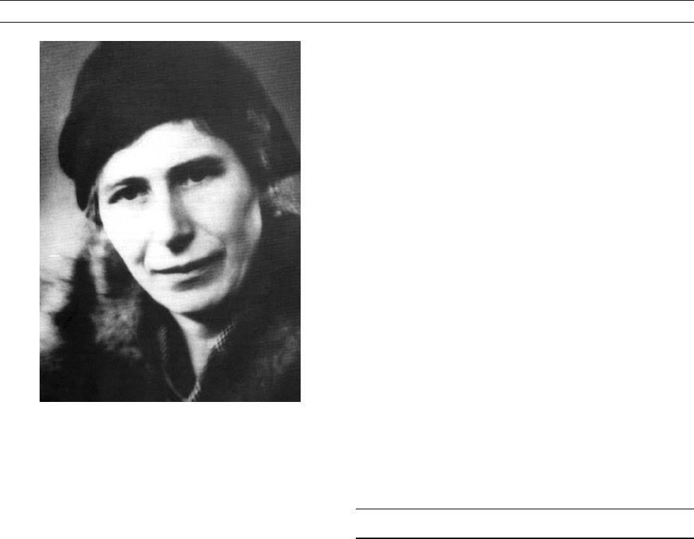
In 1936, Miss Inge Lehmann (Figure L2) proposed a new seismic shell

of radius 1400 km at the center of the Earth, which she called the

“inner core.” It was already known that low seismic velocities in the

outer core created a shadow at angular distances between 105



and

142



and that seismic waves diffracted some considerable distance into

the shadow. Wiechert also attributed seismic arrivals before 142



diffraction, but Gutenberg and Richter (1934) had already found their

468 LARMOR, JOSEPH (1857–1942)

amplitude too large and frequency too high to fit with the diffraction

theory. Measurements of the vertical component of motion clinched

the interpretation as waves reflected or refracted through a large angle.

Lehmann’s paper remains a classic example of lateral thinking, careful

interpretation, and cautious conclusions. The proposed radius was

close to the currently accepted one of 1215 km.

The inner core was rapidly accepted into the new Earth models

being constructed by Gutenberg and Richter (1938) in the United

States and Jeffreys (1939) in the U.K., although the scattered nature

of the arrivals in the shadow zone demanded a thick transition zone

at the bottom of the outer core, where the seismic velocity increased

gradually. In the first edition of his book on seismology, Bullen

(1947) labeled the Earth’s layers A-G, with A as the crust and G the

inner core, with F denoting the inner core transition. The need for this

layer was largely removed when seismic arrays showed that much of

the scattered energy came not from the inner-core boundary but from

the core-mantle boundary (Haddon and Cleary, 1974). The inner core

is vital in the theory of geomagnetism because its slow accretion, a

consequence of the Earth’s secular cooling, powers the geodynamo

and influences core convection (see Inner core tangent cylinder).

The F-layer lives on in name at least, despite the removal of seismolo-

gical evidence, in the form of the required boundary layer between the

inner and outer cores.

Although the inner core was probably the most spectacular of

Lehmann’s discoveries, she enjoyed a long and distinguished career

in seismology, remaining active throughout her long retirement. Born

in Copenhagen into a distinguished family, she benefited from an

exceptionally enlightened early education and read mathematics at

the University of Copenhagen from 1908. A spell in Cambridge in

1910 came as a shock because of the restrictions placed on women

there (Cambridge did not grant women degrees until much later).

Lehmann’s career as a seismologist began in 1925 when she was

appointed assistant to Professor N.E. Norland, who was engaged in

establishing a network of seismographs in Denmark. She met Beno

Gutenberg at this time. In 1928 she was appointed chief of the seismo-

logical department of the Royal Danish Geodetic Institute, a post she

held until retirement in 1953. In retirement she enjoyed frequent visits

to Lamont and other institutions in the United States and Canada. It

seems her international reputation was strong before her work was

recognized at home in Denmark. She was elected Foreign Member

of the Royal Society in 1969, was awarded the Bowie Medal (the

American Geophysical Union highest honor) in 1971, and now has

an AGU medal named in her honor.

Further details of her life may be found in Bolt (1997).

David Gubbins

Bibliography

Bolt, B.A., 1997. Inge Lehmann. Biographical Memoirs of Fellows of

the Royal Society, 43: 28285–28301.

Bullen, K.E., 1947. An Introduction to the Theory of Seismology.

London: Cambridge University Press.

Gutenberg, B., and Richter, C.F., 1938. P’ and the Earth’s core.

Monthly Notices of Royal Astronomical Society, Geophysical Sup-

plement, 4: 363–372.

Haddon, R.A.W., and Cleary, J.R., 1974. Evidence for scattering of

seismic PKP waves near the mantle-core boundary. Physics of the

Earth and Planetary Interiors, 8 :211–234.

Jeffreys, H., 1939. The times of the core waves. Monthly Notices of

Royal Astronomical Society, Geophysical Supplement, 4: 548–561.

Lehmann, I., 1936. Publication’s Bureau Centrale Seismologique

Internationale Series A, 14:87–115.

Cross-reference

Inner Core Tangent Cylinder

LENGTH OF DAY VARIATIONS, DECADAL

It is a truism to say that the Earth rotates once per day. However, the

length of each day is not constant, but varies over timescales from

everyday to millions of years. Perhaps the best-known variation is

the gradual slowing of the rotation rate due to the tidal interaction

between the Earth and the moon (see Length of day variations, long-

term). Historical observations are well fit by an increase in length of

day (LOD) of about 1.4 ms per century, most clearly seen in the timing

of eclipses recorded by ancient civilizations. (Note that there are

86 400 seconds in a day, so these millisecond changes are of order

1 part in 10

of the basic signal.) Geological evidence also supports

increase in LOD over Earth history (Williams, 2000). At the other end

of the scale, modern measurements from the global positioning system

(GPS) or very-long baseline interferometry (VLBI) demonstrate a sig-

nal on yearly and sub-yearly timescales, again of a few milliseconds

in magnitude. These variations are dominated by angular momentum

exchange between the atmosphere and the solid Earth; put crudely,

winds blowing against mountain topography (particularly north-south

ranges such as the Rockies in America) push the solid Earth, speeding

up or slowing down the rate of rotation. Atmospheric angular momen-

tum calculated from models of the global circulation can explain

almost all the short-period signals. The small remaining residual (of

amplitude 0.1 ms) shows strong coherence with estimates of oceanic

angular momentum (Marcus et al., 1998), and the hydrological cycle

is also probably important, by causing small variations in the Earth’s

moment of inertia. However, surface observations are unable to explain

a decadal fluctuation, again of a few milliseconds in LOD. This signal

was first recognized in the early 1950s, and because the core is the only

fluid reservoir in the Earth capable of taking up the requisite amount of

angular momentum and due to its correlation with various geomagnetic

data (in particular records of magnetic intensity and declination at cer-

tain magnetic observatories), it was assumed to result from exchange

Figure L2 Inge Lehmann (Reprinted with permission from the Royal

Society).

LENGTH OF DAY VARIATIONS, DECADAL 469

of angular momentum between the fluid core and solid mantle. More

robust evidence was provided by Vestine (1953), who demonstrated a

good correlation between the change in length of day (DLOD) signal

and core angular momentum (CAM) estimated from observations of

westward drift (q.v.).

The connection between core processes and DLOD was put on a

rigorous footing by Jault et al. (1988). They realized that models of

surface core flow reflect motions throughout the core and can be used

to estimate changes in angular momentum of the core, matching

changes in angular momentum of the solid Earth required to explain

the observed decadal DLOD. Most processes in the core have charac-

teristic timescales which are either of centuries or longer (for example

the planetary waves that have been proposed as an explanation for

westward drift (q.v.)), or which are short, of order days (Alfvén waves

(q.v.) or inertial waves). Torsional oscillations (q.v.), however, are

thought to have characteristic periods of decades. These are solid-body

rotations of fluid cylinders concentric with the Earth’s spin axis, about

that axis. Such motions carry angular momentum about the spin axis,

and extend to the core surface. Therefore, changes in CAM can be

calculated using surface flow models. Such a calculation ignores the

inner core, and assumes uniform density for the liquid core; however,

the value calculated is not sensitive to these assumptions. Most

commonly, a surface flow is used that is assumed to be tangentially

geostrophic (the force balance in the horizontal direction is assumed

to be between pressure gradients and Coriolis force). The core surface

flow is expanded in a poloidal-toroidal decomposition in spherical

coordinates (r, y, j)(ris radius, y is colatitude, and j is longitude),

such that

v ¼

l¼1

m¼0



þr

 rt



(Eq. 1)

where r

is the horizontal part of the gradient operator, and s

and t

are poloidal and toroidal scalars, respectively, corresponding to surface

spherical harmonics (q.v.) Y

ð; jÞ of degree l and order m. Then,

core angular momentum depends only on two large-scale toroidal,

zonally symmetric, surface flow harmonics. Using standard parameters

for the Earth, the relation

T ¼ 1:138 t

t



(Eq. 2)

is obtained, where dT is the change in LOD in milliseconds and the

changes in the toroidal flow coefficients are measured in km y

1

The t

harmonic corresponds to a uniform rotation of the core surface

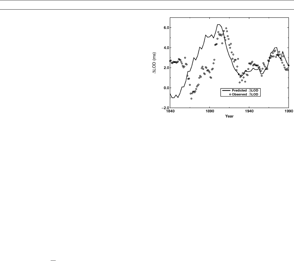
about the Earth’s rotation axis. Figure L3 shows a calculation of

Jackson et al. (1993) using the ufm time-dependent model of the main

field (q.v.) to calculate the predicted LOD variations, compared with

observations of McCarthy and Babcock (1986). Despite the highly idea-

lized theory, the agreement is striking, especially over the last century.

The correlation post-1900 between LOD and calculated core-

angular momentum is remarkably robust, being evident for many

different strengths of flow (explaining more or less of the secular var-

iation) and for different physical assumptions about the flow (for

example, assuming that the flow is toroidal, or steady but within a

drifting reference frame). By 1900 the network of magnetic observa-

tories (q.v.) was globally distributed; these stations provide by far the

most sensitive and accurate measurements of the global magnetic secu-

lar variation from which the flows are calculated. Before 1900, as

more observatory data become available, the time variation of the

field models reflects changes in data quality as well as any physical

processes; these changes map into the flow models, giving unphysical

results and poorer correlation with observed D LOD. There is some

evidence that this problem can be overcome by calculating simpler

flow models; a notably better correlation is provided by the original

analysis (Vestine, 1953) of westward drift!

More recent work has considered whether the core could have a role

to play in angular momentum exchange at shorter periods. It has been

argued that the core may well change the phase of the observed LOD

signal compared with forcing from the atmosphere and oceans, but there

is no strong evidence in subdecadal DLOD of a signal from the core.

The study of LOD variations as described here is essentially phe-

nomenological—there is no need to assume any particular mechanism

for the exchange of angular momentum between the core and the man-

tle. How the exchange of angular momentum may be effected, and the

influence of the dynamics of the torsional oscillations (q.v.), are

discussed elsewhere.

Richard Holme

Bibliography

Jackson, A., Bloxham, J., and Gubbins, D., 1993. Time-dependent

flow at the core surface and conservation of angular momentum

in the coupled core-mantle system. In Le Mouël, J.-L., Smylie,

D.E., and Herring T. (eds.), Dynamics of the Earth’s Deep Interior

and Earth Rotation, pp. 97–107, AGU/IUGG.

Jault, D., Gire, C., and Le Mouël, J.L., 1988. Westward drift, core

motions, and exchanges of angular momentum between core and

mantle. Nature, 333: 353–356.

Marcus, S.L., Chao, Y., Dickey, J.O., and Gregout, P., 1998. Detection

and modeling of nontidal oceanic effects on Earth’s rotation rate.

Science, 281: 1656–1659.

Vestine, E.H., 1953. On variations of the geomagnetic field, fluid

motions and the rate of the Earths rotation. Journal of Geophysical

Research, 38:37–59.

Williams, G.E., 2000. Geological constraints on the Precambrian

history of earth’s rotation and the moon’s orbit. Reviews of

Geophysics, 38:37–59.

Cross-references

Alfvén Waves

Core-Mantle Coupling, Electromagnetic

Core-Mantle Coupling, Topographic

Harmonics, Spherical

Length of Day Variations, Long-Term

Observatories, Overview

Oscillations, Torsional

Time-Dependent Models of the Geomagnetic Field

Westward Drift

Figure L3 Comparison of observed decadal variations in length of

day LOD (with a long-term trend of 1.4 ms/century removed) with

the prediction from a model of surface core flow (following Jackson

et al., 1993).

470 LENGTH OF DAY VARIATIONS, DECADAL

LENGTH OF DAY VARIATIONS, LONG-TERM

Tidal friction

The Moon raises tides in the oceans and solid body of the Earth. The

Sun does likewise, but to a lesser extent. Let us first consider the action

of the Moon. Due to the anelastic response of the Earth’s tides, the tidal

bulges can be thought of as being carried ahead of the sublunar point

by the Earth’s rotation. This misalignment of the tidal bulges produces

a torque on the Moon, which increases its orbital angular momentum

and drives it away from the Earth, while reducing the Earth’s rotational

angular momentum by the opposite amount. The rate of rotation of the

Earth is reduced through the action of tidal friction, which occurs very

largely in the oceans. By analogy, the solar tides make a smaller contri-

bution to slowing down the Earth, but the reciprocal effect on the Sun

is negligible. As the Earth slows down the length of the day (LOD)

increases. The change in the rate of rotation of the Earth under this

mechanism is usually termed its tidal acceleration. Beside this long-term

change, there are relative changes between the rotation of the mantle

and the core on shorter timescales. The transfer of angular momentum,

which produces these changes, is caused by core-mantle coupling and

the astronomical results discussed here shed light on the timescale of

the geomagnetic processes involved.

The tidal acceleration of the Earth has been measured reliably in the

following way. Analysis of the perturbations of near-Earth satellites

produced by lunar and solar tides, together with the requirement that

angular momentum be conserved in the Earth-Moon system, leads

to an empirical relation between the retardation of the Earth’s spin

and the observed tidal acceleration of the Moon (see, for example,

Christodoulidis et al. (1988)). Lunar laser ranging gives an accurate

value for the Moon’s tidal acceleration and inserting this in the relation

gives the result –6.1  0.4  10

22

rad s

2

for the total tidal accelera-

tion of the Earth (Stephenson and Morrison, 1995). This result is

equivalent to a rate of increase in the LOD of þ2.3  0.1 ms per cen-

tury (ms/100 y). For the interconversion of units see Table 2 of

Stephenson and Morrison (1984). These satellite and lunar laser ran-

ging measurements were obtained from data collected over the past

30 years or so. However, they can be applied to the past few millennia

because the mechanism of tidal friction has not changed significantly

during this period (see, for example, Lambeck, 1980, Section 10.5).

While the tidal component of the Earth’s acceleration can be derived

from recent high-precision observations, the actual long-term accelera-

tion, which is the sum of the tidal and nontidal components, cannot be

measured directly because it is masked by the relatively large decade

fluctuations. Instead, observations from the historical past, albeit crude

by modern standards, have to be used. By far the most accurate data

for measuring the Earth’s rotation before the advent of telescopic

observations (ca.

A.D. 1620) are records of eclipses. Useful records of

eclipses extend back to about 700

B.C.

Eclipses and the Earth’s rotation

Early eclipse observations fall into two main independent categories:

untimed reports of total solar eclipses; and timed measurements of

solar and lunar eclipse contacts. The tracks of total solar eclipses on

the Earth’s surface are narrow and distinct. The retrospective calcula-

tion of their occurrence is made by running back the Sun and Moon

in time along their apparent orbits around the Earth, the Moon’s

motion having been corrected for the lunar tidal interaction with the

Earth. Unless special provision is made, this computation presupposes

the uniform progression of time and hence the uniform rotation of the

Earth on its axis. For each observation, the displacement in longitude

between the computed position of the track of totality and the actual

observed track measures the cumulative correction to the Earth’s rota-

tional phase due to variations in its rate of rotation over the intervening

period. This displacement in degrees, divided by 15, gives the correc-

tion in hours to the Earth ’s “clock,” usually designated by DT.

Stephenson and Morrison (1995) analyzed all the available reliable

records of solar and lunar eclipses during the period 700

B.C. to A.D.

1600 from ancient Babylon, China, Arab, and European sources in

order to measure DT at epochs in the past. For full translations of the

various historical records see Stephenson (1997). The untimed data

consist of unambiguous descriptions of total solar eclipses from known

places on particular dates, but without timing. The measurement of

time is not necessary because of the narrowness of the belt of totality

(a few minutes of time) relative to the quantity being measured (DT),

which amounts to several hours in the era

B.c. The timed data, on

the other hand, include a timing of the occurrence of one or more of

the contacts during solar and lunar eclipses.

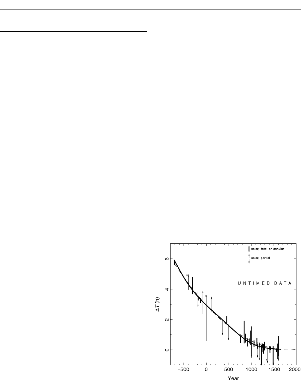
Their results for DT from the untimed data are shown in Figure L4.

Some less-critical data have been omitted here from the figure for the

sake of clarity. A single parabola does not adequately represent all the

data, so Stephenson and Morrison fitted a smooth curve to the data

using cubic splines, with economical use of knots in order to follow

the degree of smoothness in the observed record after

A.D. 1600. The

details of the fitting procedure can be found in their 1995 paper. Their

results from the independent timed data are very close to the untimed

data, and are not reproduced here.

Long-term accelerations in rotation

The parabola in Figure L4 corresponds physically to an acceleration

of –4.8  0.2  10

22

rad s

2

in the rotation of the Earth. This is sig-

nificantly less algebraic than the acceleration expected on the basis of

tidal friction alone, –6.1  0.4  10

22

rad s

2

. Some other mechan-

ism, or mechanisms, must account for the accelerative component

of þ1.3  0.4  10

22

rad s

2

. This nontidal acceleration may be

associated with the rate of change in the Earth’s oblateness attributed

to viscous rebound of the solid Earth from the decrease in load on the

polar caps following the last deglaciation about 10000 years ago (Peltier

and Wu, 1983; Pirazzoli, 1991). From an analysis of the acceleration of

the motion of the node of near-Earth satellites, a present-day fractional

Figure L4 Corrections to the Earth’s clock derived from the

differences between the observed and computed paths of

(untimed) solar eclipses. The vertical lines are not error bars, but

solution space, anywhere in which the actual value is equally

likely to lie. Arrowheads denote that the solution space extends

several hours in that direction. The solid line has been fitted by

cubic splines. The dashed line is the best-fitting parabola.

LENGTH OF DAY VARIATIONS, LONG-TERM 471

rate of change of the Earth’s second zonal harmonic J

of –2.5  0.3 

11

per year has been derived, which implies an acceleration in the

Earth’s rotation of þ1.2  0.1  10

22

rad s

2

. This is consistent to

within the errors of measurement with the result from eclipses, assuming

an exponential rate of decay of J

with a relaxation time of not less than

4000 years. Other causes may include long-term core-mantle coupling

and small variations in sea level associated with climate changes.

Long-term changes in the length of the day

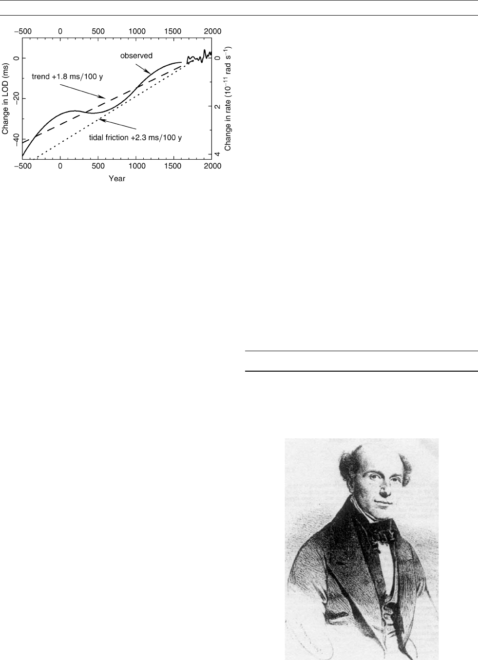
The first time-derivative along the curves in Figure L4 gives the

change in the rate of rotation of the Earth from the adopted standard.

This standard is equivalent to a LOD of 86400 SI s. The change in

the LOD is plotted in Figure L5. The wavy line is the derivative

along the cubic splines in the period 500

B.C. to A.D. 1600. After A.D.

1600, the higher resolution afforded by telescopic observations reveals

the decade fluctuations (see Length of day variations, decadal), which

are usually attributed to core-mantle coupling (see Core-mantle

coupling) (see Ponsar et al., 2003). Similar fluctuations are undoubt-

edly present throughout the whole historical record, but the accuracy

of the data is not capable of resolving them. All that can be resolved

is a long-term oscillation with a period of about 1500 years and ampli-

tude comparable to the decade fluctuations. The observed acceleration

of –4.8  0.2  10

22

rad s

2

in Figure L4 is equivalent to a trend of

þ1.8  0.1 ms/100 y in the LOD. In our considered opinion, no reli-

able eclipse data suitable for LOD determinations are available before

ca. 700

B.C.

Paleorotation

The rotation of the Earth about 400 Ma ago can, in principle, be mea-

sured from the seasonal variations in growth patterns of fossilized cor-

als and bivalves. This leads to estimates of the number of days in the

year at that time, and hence the LOD (the year changes very little).

Lambeck (1980) reviews the data and arrives at the value –5.2 

0.2  10

22

rad s

2

(¼þ1.9  0.1 ms/100 y in LOD) for the tidal

acceleration over the past 4  10

years, which implies that tidal

friction was less in the past.

L.V. Morrison and F.R. Stephenson

Bibliography

Christodoulidis, D.C., Smith, D.E., Williamson, R.G., and Klosko,

S.M., 1988. Observed tidal braking in the Earth/Moon/Sun system.

Journal of Geophysical Research, 93: 6216–6236.

Lambeck, K., 1980. The Earth’s Variable Rotation. Cambridge UK:

Cambridge University Press.

Peltier, W.R., and Wu, P., 1983. History of the Earth’s rotation. Geo-

physical Research Letters, 10: 181–184.

Pirazzoli, P.A., 1991. In Sabadini, R., Lambeck, K., and Boschi, E.

(eds.), Glacial Isostacy, Sea-level and Mantle Rheology. Dordrecht:

Kluwer, pp. 259–270.

Ponsar, S., Dehant, V., Holme, R., Jault, D., Pais, A., and Van Hoolst, T.,

2003. The core and fluctuations in the Earth’s Rotation. In

Dehant, V., Creager, K.C., Karato, S., and Zatman, S. (eds.), Earth’s

Core: Dynamics, Structure, Rotation Vol 31. Washington, DC:

American Geophysical Union Geodynamics Series, pp. 251–261.

Stephenson, F.R., 1997. Historical Eclipses and Earth’s Rotation.

Cambridge UK: Cambridge University Press.

Stephenson, F.R., and Morrison, L.V., 1984. Long-term changes in

the rotation of the Earth: 700

B.C. to A.D. 1980. In Hide, R. (ed.),

Rotation in the Solar System. The Royal Society, London.

Reprinted in Philosophical Transactions of the Royal Society of

London, Series A, 313:47–70.

Stephenson, F.R., and Morrison, L.V., 1995. Long-term fluctuations in

the Earth’s rotation: 700

B.C. to A.D 1990. Philosophical Transac-

tions of the Royal Society of London, Series A, 351: 165–202.

Cross-references

Core-Mantle Coupling-Electromagnetic

Geomagnetic Spectrum, Temporal

Halley, Edmond (1656–1742)

Length of Day Variations, Decadal

Mantle, Electrical Conductivity, Mineralogy

Westward Drift

LLOYD, HUMPHREY (1808–1881)

Humphrey Lloyd (Figure L6) was a distinguished and influential

experimental physicist whose entire career was pursued at Trinity

College, Dublin (O’Hara, 2003).

Figure L5 Changes in LOD –500 to þ2 000 obtained by taking the

first time-derivative along the curves in Figure L4. The change due

to tidal friction is þ2.3 ms/100 y. The high-frequency changes after

þ1700 are taken from Stephenson and Morrison (1984).

Figure L6 Humphrey Lloyd.

472 LLOYD, HUMPHREY (1808–1881)

In optics, he is remembered for his experimental confirmation of

Hamilton’s prediction of conical refraction, his demonstration of inter-

ference fringes with a pair of mirrors, and his authoritative report on

the wave theory of light for the British Association. He had a lifelong

interest in terrestrial magnetism and played an important role in the

establishment of magnetic observatories, beginning in the 1830s.

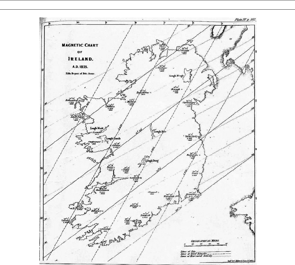
His first venture into geomagnetism was a survey of Ireland (Figure L7)

(Lloyd et al., 1836) undertaken, at the instigation of the British Asso-

ciation, with Ross and Sabine (q.v.) in 1834 and 1835. In addition to

dip and the horizontal component of the Earth’s field, measured follow-

ing the oscillation method of Hansteen (q.v.), simultaneous measure-

ments of dip and intensity were made by a static balance method of

his own devising.

Following the lead of von Humboldt (q.v.) and Gauss (q.v.) and with

the detailed advice of the latter, Lloyd proceeded to have his Magnetical

Observatory built in the grounds of the college. This charming edifice

can still be viewed, but in the grounds of University College Dublin,

some miles distant from its original home.

He conceived and designed many of the instruments that were to be

used in the observatory: most were made by Thomas Grubb of Dublin.

These included his balance magnetometer and a bifilar magnetometer,

which he had developed to measure the horizontal component.

Lloyd participated enthusiastically in Gauss’s Europe-wide Mag-

netic Union, and when such observatories came to be established

throughout the British colonies, at the urging of Sabine (q.v.)

Lloyd was heavily involved. The Dublin facility served as a model

for those far-flung stations and new observers were trained in the

college. The association of European, Russian, and British observa-

tories represented what Lloyd called “a spirit unparalleled in the

history of science.” They constituted the first global network devoted

to a scientific project. (see Observatories, overview). The specific

idea of a network for magnetic observations lives on today in

Intermagnet.

Even his honeymoon in 1840 was subsumed in the busy program of

overseas observatory visits that followed. Meanwhile his inventiveness

continued to show itself in new and refined designs for instrumenta-

tion: for example an induction magnetometer for the vertical compo-

nent (1841).

The current notion that terrestrial magnetism was linked to meteor-

ological phenomena led him to study the latter, with a characteristi-

cally systematic approach. He also explored the conjecture that

internal electric currents were responsible for the Earth’s field, tried

to relate this to the diurnal variation, and proposed new experiments

to test this theory.

Figure L7 Lloyd’s magnetic survey of Ireland, undertaken with Ross and Sabine.

LLOYD, HUMPHREY (1808–1881) 473

Lloyd’s father Bartholomew had been an inspiring leader of the col-

lege as a reforming mathematician and provost. Humphrey followed

his example in becoming provost, and served as president of the Royal

Irish Academy and the British Association. He was recognized with

such awards as the German “Pour le Mérite” and Fellowship of the

Royal Society. At home, he was awarded the Royal Irish Academy’s

Cunningham Medal.

He wrote 8 books and 64 papers and reports that record the achieve-

ments and insights of a remarkable experimentalist, organizer, and

educator. A bust and a number of portraits survive in his college. There

his father had created a new impetus in mathematics; the son accom-

plished the same for experimental science.

On his death, the Erasmus Smith Chair of Experimental and Natural

Philosophy passed to George Francis Fitzgerald, together with much of

Lloyd’s energy and ideals. He had “struck an almost twentieth century

note in his emphasis on the importance to a university of the cultiva-

tion of scientific research” (McDowell and Webb, 1982).

Deanis Weaire and J.M.D. Coey

Bibliography

Lloyd, H., Sabine, E., and Ross, J.C., 1836. Observations on the

Direction and Intensity of the Terrestrial Magnetic Force in Ireland.

In the Fifth Report of the British Association for the Advancem-

ment of Science. London: John Murray, pp. 44–51.

McDowell, R.B., and Webb, D.A., 1982. Trinity College Dublin,

1592–1952: An Academic History. London: Cambridge University

Press.

O’Hara, J.G., 2003. Humphrey Lloyd 1800–1881. In McCartney,

M., and Whitaker, A. Physicists of Ireland. Bristol: IOP Publish-

ing, pp. 44–51.

Cross-references

Gauss, Carl Friedrich (1777–1855)

Hansteen, Christopher (1784–1873)

Humboldt, Alexander von (1759–1859)

Observatories, Overview

Sabine, Edward (1788–1883)

474 LLOYD, HUMPHREY (1808–1881)

MAGNETIC ANISOTROPY, SEDIMENTARY

ROCKS AND STRAIN ALTERATION

The relationship between anisotropy of magnetic susceptibility (AMS)

fabrics (the shape and orientation of the AMS ellipsoid) and rock fab-

rics has been studied for over 40 years. Many studies have employed

magnetic fabrics as an independent data set to compare with remanent

magnetization directional data. Magnetic fabrics can also be very sen-

sitive indicators of low-intensity strain, though deformation exceeding

10% to 20% often modifies or destroys the fabric to the point of

making a functional interpretation impossible. This is in part due to

diagenetic processes; for example, reduction, pressure solution, recrys-

tallization, fluid migrations, and growth of new mineral constituents

occurring with greater degrees of strain. Thus, AMS techniques are

most often successful in investigating tectonic strains on weakly

deformed sedimentary rocks.

While AMS fabrics are most often easily interpreted in sedimentary

rocks, the method is nonetheless complicated by the great range of pri-

mary sedimentary fabrics requiring correct interpretation before any

modification to that fabric can be understood. It is important to note

that AMS ellipsoids and grain-shape often do not correspond. Recent

studies have pointed out the strong dependence of the AMS ellipsoid

shape on mineral composition, for example, which can have a much lar-

ger effect than strain modification. Slight variations in ferromagnetic (or

ferrimagnetic) trace minerals, for example, can strongly influence the

shape and magnitude of the AMS ellipsoid, to the extent that composi-

tion-dependent variation may completely obscure the effects of strain.

Finally, modeling and experimental studies have demonstrated that the

relationship between incremental strain and the change in degree of ani-

sotropy is highly complex. Some studies have determined power-law

relationships, but with a great deal of variability reflecting differences

in deformational style, intensity, and minerals that carry the anisotropy.

Despite such complications, AMS methods as fabric indicators in sedi-

mentary rocks have the advantages of being rapid, nondestructive, and

result from the averaging of a susceptibility tensor from a very large

population of magnetic grains. Weak deformation distinguished by

AMS techniques may often be undetectable by nonmagnetic methods.

Depositional (primary) sedimentary fabrics

and processes

AMS studies have been directed at analyzing deep-sea current flow, bio-

turbation, fluvial and lacustrine fabrics, wind-deposited sand and loess

fabrics, to name a few, as interpreted from AMS ellipsoids. Since

sedimentary rocks should nearly always have a primary magnetic fabric,

any fabric acquired as a result of later deformation will be superimposed

upon a preexisting depositional fabric. Therefore, interpretation of

altered AMS fabrics must begin with interpretation of the earlier

(primary) fabric, which controls any subsequent alteration.

Studies of depositional AMS fabrics in sediments show that the

shape and orientation of the susceptibility ellipsoid can be affected

by a great variety of sedimentological processes predominantly formed

during the deposition of particles from suspension in water or air (for a

review, see Ellwood, 1980). Initial sedimentary fabrics are generally

determined by gravity and hydrodynamics. Thus, to a first approxima-

tion, the shape and orientation of the AMS ellipsoid (which is the sum

of the susceptibilities of a large number of grains present in the mea-

sured sample) is determined by both the characteristics of the grains

themselves, and by the velocity and direction of transport of the med-

ium through which they are carried. In general, sedimentary deposi-

tional fabrics are comparatively low in both susceptibility (<10

–4

units) and in anisotropy (<5%). Typical primary depositional fabrics

tend to be characterized by vertical or subvertical minimum suscept-

ibility axes (K

) (that is, the magnetic foliation is near the bedding

plane) consistent with a conceptual model of grains settling flat on a

surface. The maximum susceptibility axis (K

) is often related to the

transport or postdepositional current direction. However, this simple

conceptual model can be complicated by factors such as the velocity

of grains during deposition, the angle of slope on which grains settle,

bulk mineralogy, compaction, fluid migration, and chemical changes

such as growth of authigenic minerals or oxidation of iron-containing

minerals, which may modify or completely destroy the original deposi-

tional fabric.

Many studies of deep-sea sediments have been aimed at describing

variables such as current velocity or transport mechanisms through

interpretation of the orientation of AMS ellipsoids, particularly the

orientation of the maximum susceptibility axis (K

) or the lineation

). A number of studies have successfully used AMS to orient

sediment cores used for studies of paleomagnetic remanence, and

many investigations have described and identified the degree to which

sampling techniques used for deep-sea sediments can distort the sam-

ples, thus affecting the measured AMS fabric.

In deep-sea sediments, both current-parallel and current-perpendicular

alignments of the maximum susceptibility (K

) axes are reported in

a variety of depositional environments. One might imagine that the

long axis of an elongate grain would align with current direction

like a weather vane. In rock fabric studies, however, there are many

reported instances of “rolling fabrics,” in which elongated axes of

grains are oriented perpendicular to the current direction as a result