Gubbins D., Herrero-Bervera E. Encyclopedia of Geomagnetism and Paleomagnetism

Подождите немного. Документ загружается.

which to the first approximations is reduced to

T ¼

f 

B (Eq. 3)

where

B is the unit vector in the core field direction. Almost all aero-

magnetic measurements on Earth result in magnetic anomalies as

defined in Eq. (3). In case of a planet with no core field, such as Mars,

a magnetic anomaly simply refers to the magnetic field of the litho-

sphere.

This article addresses modeling of the magnetic anomalies of the

planetary lithosphere. The first section describes the forward model-

ing, where the shape and magnetization of a magnetic body is given

and the magnetic anomaly of the body is to be determined. The second

section considers the inverse problem, where the magnetic anomalies

are measured and the shapes and magnetization of the magnetic source

bodies are to be determined.

Forward modeling

The magnetic potential V of a magnetic body is

V ð

rÞ¼

ZZZ

Mð

Þr

r 

(Eq. 4)

where m

is the magnetic permeability of free space

ð4p  10

7

1

Þ,

Mð

Þ is the magnetic dipole moment per unit

volume, called magnetization, and the integration is over the entire

volume of the body. Equation (4) is quite complicated especially when

the body is irregular in shape and has heterogeneous magnetization. In

forward modeling it is usually assumed that the magnetic body is uni-

formly magnetized in a given direction. The size and magnetization of

the source body is determined by fitting the model anomaly to the

observed one. To better fit the model field to the observation, it is often

required to divide the body into several parts with different magnetiza-

tion, but each part has still a uniform magnetization. The constant

magnetization assumption reduces Eq. (4) to

V ð

rÞ¼

r 



(Eq. 5)

upon the application of the divergence theorem.

is a surface ele-

ment and the integration is over the entire surface of the body. This

equation shows that the magnetic field outside a uniformly magnetized

body is equivalent to the magnetic field of magnetic poles (north or

south) distributed on the surface of the body. A uniformly magnetized

body acts by its surface rather than its entire volume. For example, to

determine the magnetic field of a vertically upward magnetized vertical

prism it is sufficient to assume a north pole distribution on the upper sur-

face and a south pole distribution on the bottom surface. An interesting

case is a uniformly magnetized infinite horizontal layer of constant

thickness, which produces no magnetic field outside regardless of its

magnetization intensity and direction. Such a layer is used as an annihi-

lator in the inverse problems (e.g., Parker and Huestis, 1974).

Equation (4) can also be written as

V ðrÞ¼

4prG



M r

ZZZ

r 

(Eq. 6)

for a uniformly magnetized body, where r denotes an arbitrary con-

stant density of the body and G is the gravitational constant. This

equation is further reduced to

V ðrÞ¼

4prG



M rU ð

rÞ (Eq. 7)

where

M is the unit vector of the magnetization and Uð

rÞ denotes the

gravitational potential of the body with the density r. Equation (7)

emphasis that the magnetic field outside a uniformly magnetized body

is just the gradient of the gravitational potential of the body in the

direction of its magnetization vector, with a multiplying factor

ðm

4prGÞ called the Poisson factor. This tremendously simplifies

the calculations of the magnetic field of a body, from integration of

an integrand involving vector functions to that includes only a scalar

function. A simple example is the magnetic potential of a uniformly

magnetized sphere of radius R and magnetization

centered at

which according to Eq. (7) is

V ð

rÞ¼



r

r 

(Eq. 8)

which is equivalent to the magnetic potential of a magnetic dipole

located at the center of the sphere and has a dipole moment of

Pð

Þ¼ 4p

3ðÞR

Several techniques developed in the space domain, to determine the

magnetic field of an arbitrary-shaped body, have been used for forward

modeling of an isolated magnetic anomaly (see Chapter 9 of Blakely,

1996 for details, also Telford et al., 1990). Many of the methods use

the above-mentioned characteristics of the magnetic field of a uni-

formly magnetized body. Here I briefly explain two methods; one

uses the above characteristics and the other does not. The first (e.g.,

Talwani, 1965) subdivides a magnetic body into thin horizontal slabs,

thin enough to reliably assume the walls of the slab are vertical, thus

reducing the integral in the z-direction of Eq. (4) to summation over

the slabs. The method uses the divergence theorem, a two-

dimensional version of Eq. (5), to reduce the remaining surface inte-

grals in Eq. (4) into a single line integral, the line describes the circum-

ference of the slab, which is approximated by a polygon for easy

integration. This method has been extensively used in aeromagnetic

and satellite magnetic anomaly modeling (e.g., Plouff, 1976). A simple

example of this method is the vertical prism discussed above. Because

the magnetic body is divided into many thin slabs, the method can also

handle a magnetic body with depth-dependent magnetization. The

other method is the dipole array method where a magnetic body is sub-

divided into small volume elements, small enough to approximate the

magnetization inside a volume element by a constant vector and the

magnetic field of the volume element by that of a magnetic dipole

located at the center of the volume element. This method does not

require a uniform magnetic body, because it is always possible to sub-

divide the body into very many small volume elements of constant

magnetization. Although the formulation in the rectangular coordinate

system is straightforward, there has been some incorrect formulation in

spherical coordinate system (see Dyment and Arkani-Hamed, 1998 for

details). The dipole array method has been used in modeling satellite

magnetic anomalies of Earth and Mars, where dipole arrays are placed

on the surface of the planets (e.g., Mayhew, 1979; Purucker et al.,

2000; Langlais et al., 2004). The space-domain methods, including

the two explained, generally require a huge amount of mathematical

manipulations and computer time. But the main problem with these

methods is that they do not provide insight to the general relationship

between the magnetic anomalies and the magnetization of the crust,

that the magnetic anomalies arise from lateral variations of the verti-

cally integrated magnetization. This is an important issue for under-

standing the resolving power of magnetic data. The advantage of the

space-domain methods is the sharp boundaries of the model magnetic

bodies. This enables us to integrate magnetic data with other geophysical

data, such as seismic, and obtain a better model for a given magnetic

anomaly. The Fourier domain methods, on the contrary, yield lateral var-

iations of the magnetization where boundaries of the magnetic bodies are

not sharply defined.

In the following I explain the Fourier domain technique used in

forward modeling. The Fourier domain formulation better presents

486 MAGNETIC ANOMALIES, MODELING

the relationship between the magnetization of the body and its

magnetic field.

Consider a magnetic layer of magnetization

Mð

Þ with an upper sur-

face S

and a lower surface S

. The surfaces are piecewise continuous.

In a rectangular coordinate system with the z-axis upward, Eq. (4) is

written as

V ð

rÞ¼



1

Mð

Þr

r 



(Eq. 9)

Taking two-dimensional Fourier transform of this equation yields

(Arkani-Hamed and Strangway, 1986)

x

¼

Kz

b 

x

(Eq. 10)

where

b ¼ðix; i; KÞ (Eq. 11)

and

K ¼ðx

þ 

1=2

(Eq. 12)

is the two-dimensional wave number and x and  are wave numbers is

the x and y directions.

x

is the Fourier transform of

a ¼

: (Eq. 13)

Equations (10) and (13) show that the magnetic anomaly arises from

the lateral variations of the bulk magnetization (the vertically inte-

grated magnetization) of the source body, rather than detailed varia-

tions of magnetization with depth. In a local region where the

Fourier domain formulation is applicable the core field has almost a

constant direction

. The Fourier transform of the magnetic anomaly

is then reduced to

x

¼ð



bÞV

x

(Eq. 14)

Therefore, the main task is to determine the magnetic potential of a

body.

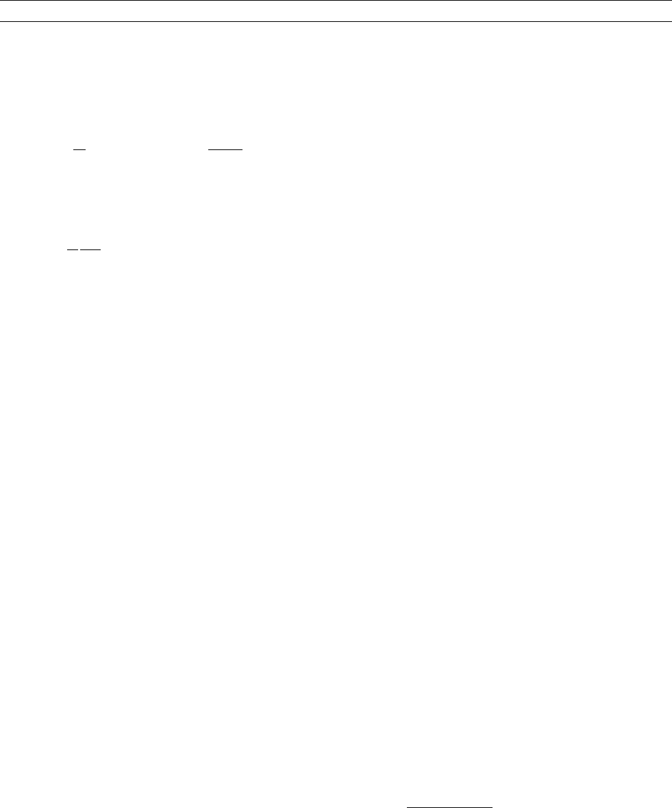
Figure M10 shows the magnetic anomaly of a rectangular body with

a square horizontal cross section of 1  1 km and a thickness of

100 m. The top of the prism is at the surface and its sides are in the

east and north directions. The body is located at the geomagnetic north

pole (column 1), at 45



N geomagnetic latitude (column 2), and at the

geomagnetic equator (column 3). It is magnetized in the direction of

the core field with an intensity of 1 A m

–1

. The magnetic anomalies are

calculated at 100 m (row 1), 500 m (row 2), and 1 km (row 3) altitudes.

The figure illustrates the complex characteristics of the magnetic

anomaly that change drastically with the body location and the obser-

vation elevation. At the 100 m elevation the anomaly delineates the

edges of the body, all the four edges at the north, only the north and

south edges at the equator, and mainly the north and south edges at



N but slightly shifted. As the elevation increases the anomalies over

the edges migrate toward the center and finally merge to give rise to a

single positive anomaly at the north, a single negative anomaly at the

equator, but a skewed anomaly at 45



N. The anomaly is directly over

the body at the north and at the equator, but is significantly shifted

toward the equator at 45



N. Moreover, the amplitude of the anomaly

changes as the body moves from the pole toward the equator. This is

due to the changes in the direction of the geomagnetic field, and thus

the magnetization. In practice the magnetization intensity, which is

assumed constant in these examples also decreases at lower latitudes,

because of the decrease in the intensity of the magnetizing geomagnetic

field.

The difficulty in relating the magnetic anomalies to their source

bodies (Figure M10) is usually alleviated by applying a reduction-to-

pole operator that reduces an anomaly to that as if the body is located

at the north pole and is magnetized by the geomagnetic field there

(e.g., Baranov, 1957; Bhattacharyya, 1965). That is, the anomalies

seen in column 2 are reduced to those in column 1. On a regional

scale where the core field direction and intensity change appreci-

ably over the entire map a differential reduction-to-pole operator

(Arkani-Hamed, 1988) is required to take into account these changes.

However, all reduction-to-pole operators are singular at the geomag-

netic equator and cannot be used to reduce the anomalies in column

3 to those in column 1.

Inverse modeling

The inverse modeling of a local magnetic anomaly map is simplified

because the core field is constant over the entire map. Blakely

(1996) discusses this issue in a great detail. However, the inverse mod-

eling of a global map is quite complicated. This is largely due to the

fact that the direction and intensity of the core field drastically change

over the globe (see Figure M10). Unlike the gravity anomaly of a body

that attains the same maximum value directly over the body regardless

of its location, the magnetic anomaly has quite complex characteris-

tics, which is a source of great confusion among those who treat the

magnetic anomaly maps similar to the gravity anomaly maps.

Here I briefly discuss major points of a generalized inversion tech-

nique developed by Arkani-Hamed and Dyment (1996) under the

assumption that the anomalies arise from the induced magnetization,

which is largely the case in the continents (e.g., Schnetzler and

Allenby, 1983). It takes into account the global variations of the core

field and transforms a global magnetic anomaly map into a global

magnetic susceptibility contrast map of the lithosphere. Unlike the

magnetic anomaly map, the magnetic susceptibility contrast map

delineates the very nature of the magnetic properties of the lithosphere.

Even a magnetization map does not delineate the nature of the mag-

netic lithosphere, because it is resulted from the multiplication of the

magnetic susceptibility and the core field intensity which changes by

more than a factor of 2 over the globe. The geomagnetic coordinate

system is adopted throughout this inversion technique and the techni-

que is based on spherical harmonic representations of the magnetic

anomalies and the magnetic susceptibility distribution, which are the

natural presentations on a global scale.

Let V be the magnetic potential of the lithosphere at an observation

point ~r, and

B denote the unit vector in the core field direction at that

point. The magnetic anomaly T is

T ¼

B rV (Eq. 15)

Let

be the unit vector along the dipole component of the core

field,

¼

ð2 cos y

r þ sin y

yÞ

ð1 þ 3 cos

yÞ

1=2

(Eq. 16)

and write

B ¼

dB (Eq. 17)

where

r and

y are the unit vectors in the r and the colatitude y direc-

tions, respectively, and

dB denotes the contribution to

B from the non-

dipole part of the core field. Also, let

MAGNETIC ANOMALIES, MODELING 487

t ¼ð1 þ 3 cos

yÞ

1=2

T (Eq. 18)

and

A ¼ð1 þ 3 cos

yÞ

1=2

dB rV (Eq. 19)

A is a measure of the contribution to the magnetic anomalies arising

from the coupling of the nondipole part of the core field with the mag-

netic potential of the lithosphere. Now expanding V, t, and A in terms

of the spherical harmonics, and putting Eqs. (16)–(19) into Eq. (15)

yields coupled equations that are solved iteratively to determine the

spherical harmonic coefficients of the magnetic potential using those

of the observed magnetic anomalies. It is worth noting, however, that

the inversion from a global magnetic anomaly map to a magnetic poten-

tial map is unstable if the core field is dipolar (Backus, 1970). Although

the entire core field is used in the calculations, the strong dominance of

the dipole component of the core field still tends to enhance the sectorial

harmonics of the potential, though slightly.

The next step is to calculate the magnetic susceptibility contrasts in

the lithosphere from the magnetic potential thus obtained. Let sð

denote the magnetic susceptibility of a volume element dv

located

at the point

in the lithosphere, then the induced magnetization of

the volume element

Mð

Þ is

Mð

Þ¼

sð

Þdv

(Eq. 20)

in which

ðr

Þ is the core field at that point. As mentioned earlier, the

most one can achieve is to determine the vertically (radially) averaged

magnetization of the lithosphere regardless of the technique used. This

is the fundamental nonuniqueness of the inversion of magnetic anoma-

lies. Therefore, we model the magnetic part of the lithosphere by a thin

Figure M10 Magnetic anomaly of a vertical prism of 1  1 km square cross section and 100 m thickness, having 1 A m

–1

magnetization. The first column shows the anomalies at the north pole, the second column shows the anomalies at 45



N latitude, and

the third column shows the anomalies at the equator. The first row shows the anomalies at 100 m, the second row at 500 m, and the

third row at 1000 m elevations.

488 MAGNETIC ANOMALIES, MODELING

magnetic spherical shell, and seek for a vertically averaged magnetic

susceptibility, i.e., we let

sð

Þ¼s

ðy

; f

Þ (Eq. 21)

Similarly, the core field is assumed to be constant with depth within

the shell, i.e.,

ð~r

Þ¼

ðy

; f

Þ (Eq. 22)

The core field intensity changes by less than 3% in the upper 50 km of

the Earth and its direction hardly changes with depth in this region.

Now decomposing

into a dipole part,

, and a nondipole part,

(Eq. 23)

and letting W denote the magnetic potential of the shell arising from

the magnetization induced by the nondipole part of the core field, we

obtain

W ¼

ðy

; f

ðy

; f

Þr

r 

(Eq. 24)

Expanding s and W in spherical harmonic and putting Eqs. (20)–(24)

into Eq. (4) results again in coupled equations that are solved

iteratively for the spherical harmonic coefficients of the magnetic

susceptibility contrast from those of the magnetic potential.

The coupled equations that are iteratively solved for the magnetic

potential using the magnetic anomaly, and for the magnetic suscept-

ibility contrast using the magnetic potential, show that the spherical

harmonic coefficients of different degrees of the magnetic susceptibil-

ity contrasts couple to those of the core field to produce a given

spherical harmonic coefficient of the observed magnetic anomalies.

This is a fundamental characteristic of a nonlinear inverse problem.

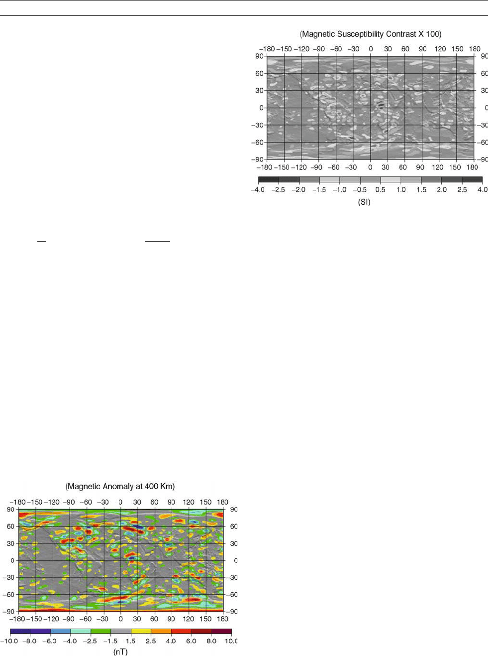
The above inversion technique is applied to the global magnetic

anomaly map of the Earth (Figure M11/Plate 6a) derived from POGO

and Magsat data that includes the spherical harmonics of degree 15–60

(Arkani-Hamed et al., 1994). The harmonic coefficients of the mag-

netic anomalies with degree lower than 15 are dominated by the core

field, and those higher than 60 are largely of nonlithospheric origin.

The magnetic lithosphere is modeled by a spherical shell of thickness

40 km. Figure M12/Plate 6b shows the resulting vertically averaged

magnetic susceptibility contrasts. Detailed interpretation of the features

seen in the figure is beyond the scope of this article. Here some basic

characteristics of the susceptibility contrast map that illustrate the

effects of the inversion process are briefly explained.

Comparison of Figures M11/Plate 6a and M12/Plate 6b shows the

major effects of the inversion. The anomalies near the polar regions

have retained their sign, whereas the anomalies in the equatorial region

have changed their sign. The magnetic susceptibility contrasts asso-

ciated with the magnetic anomalies in the midlatitudes are shifted pole-

ward with respect to the magnetic anomalies. Moreover, the amplitude

of the magnetic anomalies near the poles is significantly greater than

those in the equatorial region, whereas the magnetic susceptibilities

of their source bodies are comparable. Also, the inversion procedure

in effect includes downward continuation. The higher degree harmo-

nics of the resulting magnetic susceptibility contrast map have

enhanced compared to the corresponding harmonics of the magnetic

anomaly map at satellite altitudes. Consequently, some of the broad

features in the anomaly map are divided into two or more small size

features in the susceptibility contrast map.

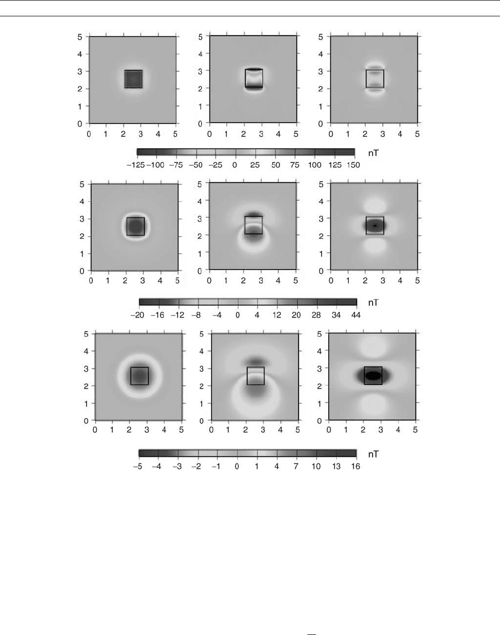
It is worth reminding that Figure M12/Plate 6b shows the vertically

averaged magnetic susceptibility contrasts within a spherical shell of

40 km thickness that can give rise to the magnetic anomalies seen in

Figure M11/Plate 6a. Figure M12/Plate 6b shows the contrasts rather

than the absolute magnetic susceptibility. The areas with positive

and negative susceptibility contrasts should be regarded as the high-

and low-magnetic areas. A constant magnetic susceptibility is usually

added to the resulting susceptibility contrast map to render all values

positive, without affecting the observed magnetic anomalies. This is

due to the fact that a spherical shell of uniform magnetic susceptibility

produces no magnetic anomaly when magnetized by an internal mag-

netic field such as the core field (Runcorn, 1975). The nonuniqueness

of the inverse problem in magnetic anomaly modeling, which is dis-

cussed in detail by Arkani-Hamed and Dyment (1996, see their

Appendix B), concludes a large range of susceptibility distribution that

give rise to no magnetic anomalies outside the lithosphere. The Run-

corn model is one of the simple cases. These susceptibility distribu-

tions can be added to a resulting susceptibility map without affecting

the resulting magnetic anomaly map.

Conclusions

This article presents both forward and inverse modeling of magnetic

anomalies. In the forward modeling the basic characteristics of

the anomalies are discussed in some detail, and a Fourier domain

technique is presented in detail. The magnetic anomaly of a vertical

Figure M11/Plate 6a Magnetic anomaly of the Earth’s lithosphere

at 400 km altitude derived from POGO and Magsat data (Arkani-

Hamed et al., 1994).

Figure M12/Plate 6b Magnetic susceptibility contrasts of a 40 km

thick spherical shell in the upper part of the lithosphere required

to give rise to the anomalies seen in Figure M11/Plate 6a.

MAGNETIC ANOMALIES, MODELING 489

prism of square cross section is shown at three elevations and at three

latitude locations, to illustrate its complex behavior. The inversion of a

global magnetic anomaly map into a global magnetic susceptibility

contrasts map consists of two nonlinear operations. The first inverts

a magnetic anomaly map into a magnetic potential map, while the sec-

ond transforms the potential map into a magnetic susceptibility con-

trast map. The nonlinearity arises from the variations in the direction

and intensity of the core field over the globe. The inversion technique

removes the adverse effects of these variations, and results in the mag-

netic susceptibility contrasts that represent the very nature of the verti-

cally averaged magnetic properties of the lithosphere.

Acknowledgment

This research was supported by the Natural Sciences and Engineering

Research Council (NSERC) of Canada.

Jafar Arkani-Hamed

Bibliography

Arkani-Hamed, J., 1988. Differential reduction to the pole of regional

magnetic anomalies. Geophysics, 53: 1592– 1600.

Arkani-Hamed, J., and Dyment, J., 1996. Magnetic potential and mag-

netization contrast of Earth’s lithosphere. Journal of Geophysical

Research, 101: 11,401–11,425.

Arkani-Hamed, J., and Strangway, D.W., 1986. Magnetic susceptibil-

ity anomalies of lithosphere beneath eastern Europe and the Middle

East. Geophysics, 51: 1711–1724.

Arkani-Hamed, J., Langel, A.L., and Purucker, M., 1994. Scalar mag-

netic anomaly maps of Earth derived from POGO and Magsat data.

Journal of Geophysical Research, 99: 24075–24090.

Backus, G.E., 1970. Non-uniqueness of the external geomagnetic field

determined by surface intensity measurements. Journal of Geophy-

sical Research, 75: 6339–6341.

Baranov, V., 1957. A new method for interpretation of aeromagnetic

maps: pseudo-gravimetric anomalies. Geophysics, 22: 359–383.

Bhattacharyya, B.K., 1965. Two-dimensional harmonic analysis as a

tool for magnetic interpretation. Geophysics, 30: 829–857.

Blakely, R., 1996. Potential Theory in Gravity and Magnetic Applica-

tions. Cambridge: Cambridge University Press.

Dyment, J., and Arkani-Hamed, J., 1998. Equivalent source magnetic

dipoles revisited. Geophysical Research Letters, 25: 2003–2006.

Langlais, B., Purucker, M.E., and Mandea, M., 2004. Crustal magnetic

field of Mars. Journal of Geophysical Research, 109: E02008,

doi:10.1029/2003JE002048.

Mayhew, M.A., 1979. Inversion of satellite magnetic anomaly data.

Journal of Geophysical Research, 45:119–128.

Parker, R.L., and Huestis, S.P., 1974. The inversion of magnetic

anomalies in the presence of topography. Journal of Geophysical

Research, 79: 1587–1593.

Plouff, D., 1976. Gravity and magnetic fields of polygonal prisms

and application to magnetic terrain corrections. Geophysics, 41:

727

–741.

Purucker, M.E., Ravat, D., Frey, H., Voorhies, C., Sabaka, T., and Acuna,

M., 2000. An altitude normalized magnetic map of Mars and its inter-

pretation. Geophysical Research Letters, 27:2449–2452.

Runcorn, S.K., 1975. On the interpretations of lunar magnetism.

Physics of the Earth and Planetary Interiors, 10: 327– 335.

Schnetzler, C.C., and Allenby, R.J., 1983. Estimation of lower crustal

magnetization from satellite derived anomaly field. Tectonophysics,

93:33– 45.

Talwani, M., 1965. Computation with the help of a digital computer

of magnetic anomalies caused by bodies of arbitrary shape. Geo-

physics, 30: 797–817.

Telford, W.M., Geldard, L.P., and Sheriff, R.E., 1990. Applied Geo-

physics, 2nd edn. New York: Cambridge University Press.

MAGNETIC DOMAINS

Introduction

The existence of a paleomagnetic record testifies to the ability of mag-

netic minerals in rocks to retain their natural remanent magnetizations

(NRMs) over geologic time. In the early days of paleomagnetism, it

was thought that the stable components of NRM mainly resided in

extremely small magnetic mineral grains, which occupied the single-

domain (SD) state. However, it is now recognized that, due to their

very small size and scarcity, SD particles may not be the major carriers

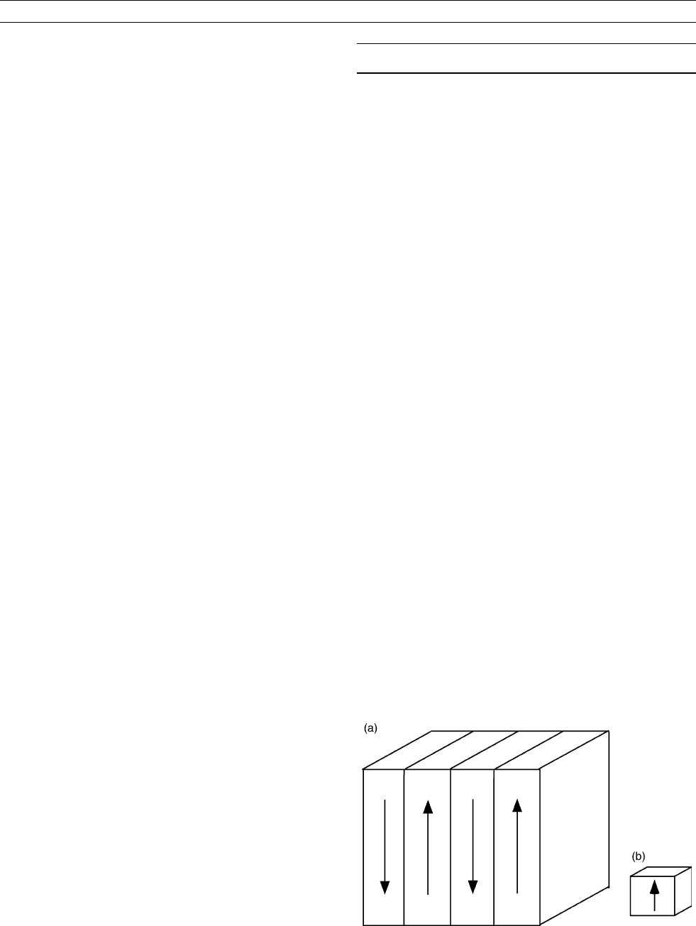
of NRM in many rocks. Instead, it is more likely that much of the

NRM is carried by grains which, by virtue of their larger sizes, are

subdivided into two or more magnetic domains (Figure M13).

For a component of NRM to survive over geologic time, a particle’s

domain structure must remain stable in two ways. First, the initial do-

main state, whether it consists of a single domain or several domains,

must resist being reset by the various physical and chemical forces

which can affect a rock after emplacement, such as moderately ele-

vated temperature, moderate pressure, slight chemical alteration, and

shifts in the direction and magnitude of the Earth’s field. In short,

the fundamental domain structure—that is, the number of domains

and the overall geometric style in which they are arranged in a crys-

tal—should not change greatly over time. Second, in particles consist-

ing of two or more domains, the domain walls (the transition regions

between adjacent domains) present initially must remain locked in

their positions, despite the aforementioned perturbations. Likewise,

coercivities in a population of SD particles must remain sufficiently high

over geologic time, so that paleomagnetic directions are not lost. Thus,

magnetic domain structure lies at the heart of paleomagnetic stability.

In this article, we first discuss some of the fundamental principles

and theoretical results of both classical magnetic domain theory and

more recent micromagnetic models. Next, we discuss results of experi-

ments to investigate how domain structure depends on grain size,

applied field, and temperature in natural magnetic minerals and their

synthetic analogs. Here, we focus on particles that contain two or more

domains, such particles being prevalent in most rocks. For more

detailed treatments of these subjects, the reader is referred to standard

texts such as Chikazumi (1964), Cullity (1972), Stacey and Banerjee

(1974), Dunlop and Özdemir (1997), and other references listed at

the end of this article.

Classical theory of magnetic domain structure

Theories of magnetic domain structure are based on three energies:

exchange energy, anisotropy energy, and magnetostatic energy. In most

Figure M13 Illustrations of (a) a multidomain cube containing

four domains and (b) a single-domain cube of uniform

magnetization.

490 MAGNETIC DOMAINS

classical theories, the first two energies produce the surface energy of

the domain wall. Magnetostatic energy, the third energy, is the poten-

tial energy required to assemble an array of “magnetic free poles”

where magnetic spins terminate at the domains’ surfaces. Magneto-

static energy is the fundamental reason why particles subdivide into

two or more domains because, in so doing, magnetostatic energy is

reduced. However, as discussed below, this subdivision carries an

energy “price”: the energy of domain walls. Consequently, below a

certain transition size particles occupy the SD state. Above this size,

particles normally contain two or more domains, the number of which

generally increases with the size of the particle. In this section, we dis-

cuss how traditional theories predict and how domain structure in a

given material depends on grain size and temperature.

Exchange energy

The origin of permanent magnetism was originally postulated by

Weiss (1907) in terms of a “molecular field” that promotes the align-

ment of atomic spins in a ferromagnetic material. Subsequently, the

molecular field was shown to be the phenomenological expression of

a quantum-mechanical phenomenon, called the exchange interaction.

Seminal calculations by Heisenberg (1928) demonstrated that the

exchange energy between two adjacent spin vectors S

and S

given by

¼2J

 S

¼2J

cos y

Here, J

is the exchange integral of the specific material and y

the angle between the two adjacent spins. In the vast majority of

natural and synthetic elements and compounds, the exchange integral

is negative; in this case, adjacent spins which are antiparallel yield

the configuration of lowest energy. Such materials are incapable

of permanent magnetism. In those few materials whose exchange inte-

gral is positive, the configuration of lowest energy is achieved when

neighboring spins are aligned. This gives rise to the rare phenomenon

of spontaneous magnetization (M

) and remanence. Such materials

possess a Curie temperature, at which spontaneous magnetism vanishes,

because (a) thermal agitation disrupts the alignment of adjacent spins,

and (b) thermal expansion of the lattice increases interatomic (or inter-

molecular) distances and thus reduces the effective strength of E

Magnetocrystalline anisotropy energy

Magnetic anisotropy causes magnetic properties to depend on the

direction in which they are measured. For example, due to magneto-

crystalline anisotropy, it requires a lower field to saturate a magnetite

crystal along the <111> directions than along <100>. Magnetocrys-

talline anisotropy arises from the coupling between spins and orbits of

the electrons. Thus, work is required to rotate spins out of the direc-

tions of lowest energy determined by spin-orbit coupling. These crys-

tallographic directions of lowest energy are often referred to as “easy”

directions of magnetization, whereas the directions of highest energy

are the “hard” directions. Easy and hard directions depend on the spe-

cific material and its crystal structure. In hexagonal crystals, for exam-

ple, the work per unit volume required to rotate the spontaneous

magnetization vector M

away from the c-axis through an angle y is:

E ¼ K

þ K

sin

y þ K

sin

y þhigher order terms:

Here, K

, K

are the material’s magnetocrystalline anisotropy con-

stants (units of erg cm

–3

in cgs). When K

> 0 and K

> K

, the

c-axis is the easy direction of magnetization, as in cobalt.

In a cubic material, the magnetocrystalline anisotropy energy den-

sity is given by:

E ¼ K

þ K

ða

þ a

ÞþK

ða

Þþ

higher order terms:

Here, a

, a

, and a

are the direction cosines of the angles between

the spontaneous magnetization vector M

and the crystal axes [100],

[010], and [001], respectively. Often, K

is much larger than K

, so that

higher powers in the expression above can be neglected. In materials

such as magnetite, both K

and K

are negative at and above room

temperature; this results in <111> being easy directions. When

> 0 and K

¼ 0, then <100> are easy directions, as in iron

(e.g., see Chikazumi, 1964; Cullity, 1972).

Stress anisotropy

Also due to spin-orbit coupling, the lattice of a ferromagnetic material

will spontaneously strain below the Curie temperature. Conversely,

application of external stress or accumulation of internal strain can

rotate the spontaneous magnetization away from the easy direction

given by crystalline anisotropy. In a cubic material the energy resulting

from an applied stress s is

E ¼3=2l

100

sða

þ a

Þ3l

111

sða

þ a

where a

, a

, and a

are the direction cosines of M

with respect to

[100], [010], and [001], respectively. The g

are the equivalent direc-

tion cosines of s; l

100

and l

111

are the material’s magnetostriction con-

stants. Tension is assumed to be positive. When l

100

¼ l

111

, as in the

case of isotropic magnetostriction, then the magnetoelastic energy

reduces to the simple form

E ¼ 3=2ls sin

where y is the angle between M

and s and where l ¼ l

100

¼ l

111

In this simple case, energy is minimum when (a) M

is parallel to s

and ls > 0 or (b) M

is perpendicular to s and ls < 0. Thus in case

(a) the application of stress will cause M

to rotate toward the stress

axis, whereas in case (b) M

will rotate toward the direction perpendi-

cular to the axis of stress.

Magnetostatic energy

The work, per unit volume, required to assemble a population of

magnetic “free poles” into a particular configuration is called the

magnetostatic energy. Magnetostatic calculations even for the simplest

domain configurations are complex and usually require numerical

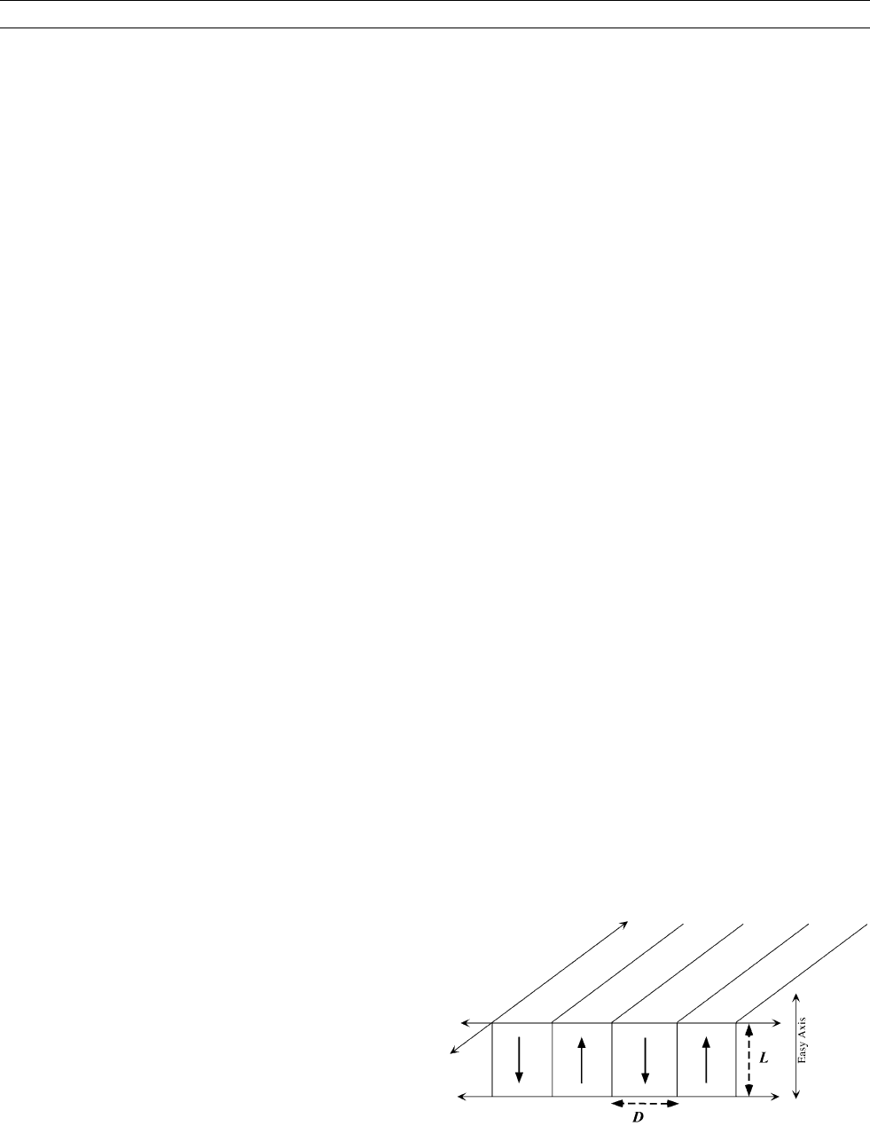
methods. One of the simplest examples was addressed by Kittel

(1949), who analyzed a semi-infinite plate of thickness L that con-

tained lamellar domains of uniform width D, with spontaneous magne-

tizations normal to the plate surface (Figure M14). Walls were

Figure M14 Illustration of the semi-infinite, magnetized plate of

thickness L, whose magnetostatic energy was calculated by Kittel

(1949). The plate contains domains of identical width D, with

magnetizations perpendicular to the plate’s surface. Walls are

assumed to be infinitely thin.

MAGNETIC DOMAINS 491

assumed to be of negligible thickness with respect to the domains’

widths and, therefore, the magnetostatic energies due to the walls’

magnetic moments were not taken into consideration.

Using the magnetic potential and a Fourier series approach, Kittel

obtained E

¼ 1.705 M

D,whereE

is the magnetostatic energy,

per unit area of plate surface (erg cm

–2

,incgs).

Note, however, that the expression above is an approximation,

because Kittel did not account for magnetostatic interactions among

all combinations of polarized slabs on the top and bottom surfaces of

the plate. Subsequently, these extra energies were included in calcula-

tions by Rhodes and Rowlands (1954). Also, they relaxed the assump-

tion of semi-infinite geometry and addressed finite, rectangular grains.

Their numerical calculations yielded “Rhodes and Rowlands” func-

tions, with which one may calculate the total magnetostatic energy

of rectangular grains of specified relative dimensions.

Energy and width of the domain wall

In the classical sense, a domain wall is the transition region where the

spontaneous magnetization changes direction from one domain to the

next. According to classical theories, each domain is spontaneously

magnetized in one direction and is clearly distinct from the wall.

(Micromagnetic theories relax this assumption and will be discussed

in a later section.)

The two most important energies that affect the domain wall’s

energy and width are (1) exchange energy and (2) anisotropy energy,

the latter being due either to magnetocrystalline anisotropy or stress.

The magnetostatic energy of the wall itself also plays a role; this

energy was first analyzed by Amar (1958) and grows especially impor-

tant when the wall width approaches that of the particle.

Were magnetocrystalline energy acting alone, the spin vectors

would change directions abruptly from one domain to the next. For

example, if a substance possessed very strong, uniaxial crystalline ani-

sotropy and exchange energy was very much weaker, then the lowest

energy “transition” between two adjacent domains would virtually

consist of two adjacent spins pointing 180



apart.

This kind of abrupt transition usually involves a large amount of

exchange energy, however, because exchange energy is minimized

when adjacent spins are parallel. Because minimization of anisotropy

energy alone would produce an infinitely thin wall, while minimiza-

tion of exchange energy alone would produce an infinitely broad wall,

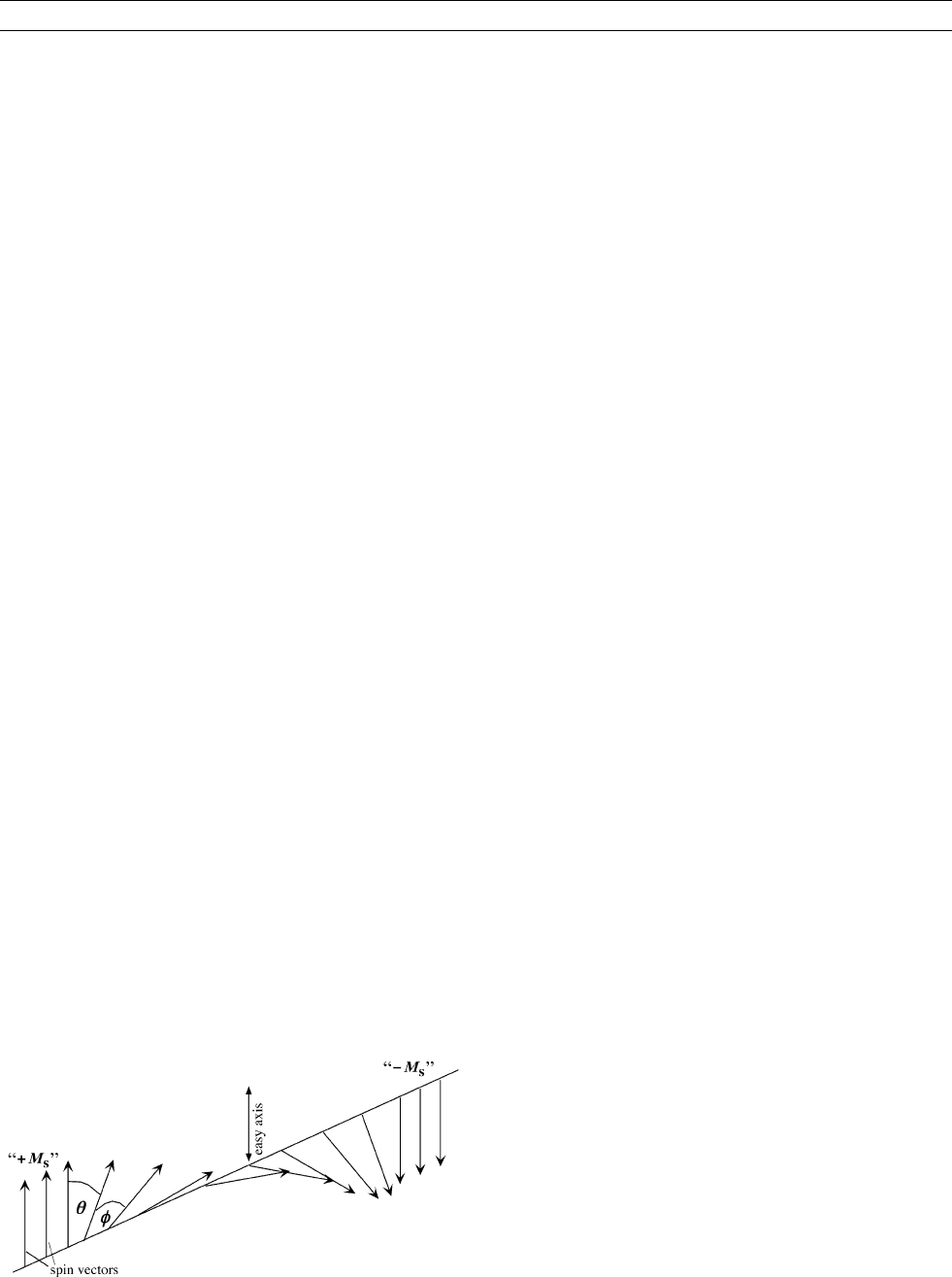
the spins in a wall rotate gradually from one domain to the next (Fig-

ure M15). This produces a wall with finite width.

By this model, spins in a wall reach an equilibrium configuration

when magnetocrystalline and exchange energies are balanced. For

the 180



Bloch wall shown in Figure M15 in which the spins rotate

through 180



, the wall energy per unit area of wall surface is

¼ 2ðJ

K=aÞ

1=2

¼ 2pðAKÞ

1=2

where J

is exchange integral, S is spin, K is anisotropy constant due

to magnetocrystalline anisotropy energy and/or stress energy, A is

exchange constant (equal to J

/a), and a is lattice constant. The

width of a 180



wall is

¼ðJS

=KaÞ

1=2

¼ pðA=KÞ

1=2

In magnetite, values predicted for E

and d

are approximately

0.9 erg cm

–2

and 0.3 mm, respectively (e.g., see Dunlop and Özdemir,

1997).

Domain width versus grain size

For the simple, planar domain structure illustrated in Figure M14,

domain width D can be calculated for the lowest energy state by mini-

mizing the sum of magnetostatic and wall energies per unit volume of

material. One obtains the familiar half-power law derived originally by

Kittel (1949):

D ¼ð1=M

ÞðE

L=1:705Þ

1=2

By this model, domain width increases with the half-power of crystal

thickness, so long as the crystal occupies the state of absolute mini-

mum energy. Experimental determinations of domain width versus

grain thickness will be discussed in a subsequent section.

Rocks, however, rarely contain magnetic minerals in the shape of

thin platelets that might be fair approximations to the semi-infinite

plate of Kittel’s model. Moskowitz and Halgedahl (1987) calculated

the number of domains versus grain size in rectangular particles

of x ¼ 0.6 titanomagnetite (“TM60”:Fe

2.4

) containing planar

domains separated by 180



walls. Magnetostatic energy, including

that due to the walls’ moments, was determined with the method devel-

oped by Amar (1958), based on Rhodes and Rowlands’ method (1954).

It was assumed that grains occupied states of absolute minimum

energy. The effects of two dominant anisotropies were investigated:

magnetocrystalline anisotropy (zero stress) and a uniaxial stress

(s ¼ 100 MPa) which was strong enough to completely outweigh

the crystalline term. Their calculations yielded two principal results:

(1) particles encompassing a wide range of grain sizes can contain

the same number of domains, and (2) a plot of N (number of

domains) versus L (grain thickness) is fitted well by a power law

N / L

1/2

. It follows that domain width D also follows a half-power

law in L. Thus, the general form of functional dependence of D on

L is the same for finite, rectangular grains, and semi-infinite plates.

Single-domain/two-dom ain transition size

Grains containing only two or three domains can rival the remanences

and coercivities of SD grains, and such particles are referred to as

being “pseudosingle-domain,” or PSD. PSD grains can be common

in many rocks and, in terms of interpreting rock magnetic behavior,

it is important to know their size ranges in different magnetic minerals.

The onset of PSD behavior begins at the single-domain–two-domain

transition size, d

In general, a particle will favor a two-domain over a SD state because

the magnetostatic energy associated with two domains is much lower

than that of a saturated particle. However, below d

the energy price

of adding a domain wall is too great to produce a state of minimum

energy. At d

the total energy of the two-domain state (E

) and the

SD state are equal; above d

, E

< E

, while E

> E

below it.

In zero applied field this transition size depends on the material’s

magnetic properties, its state of stress, the particle shape, and tempera-

ture. Moskowitz and Banerjee (1979) calculated total energies of SD,

two-domain, and three-domain cubes of stress-free magnetite contain-

ing lamellar domains at room temperature. Magnetostatic energy of the

walls was included in their calculations (Amar, 1958). They obtained

 0.08 mm.

Figure M15 Illustration of spins in a 180



Bloch wall. y is the

angle between a spin and the easy axis of magnetization; f is the

angle between adjacent spins.

492 MAGNETIC DOMAINS

Similar calculations for TM60 by Moskowitz and Halgedahl (1987)

yielded d

 0.5 mm for unstressed particles at room temperature.

Raising the stress level to 100 MPa shifted d

upward to 1 mm.

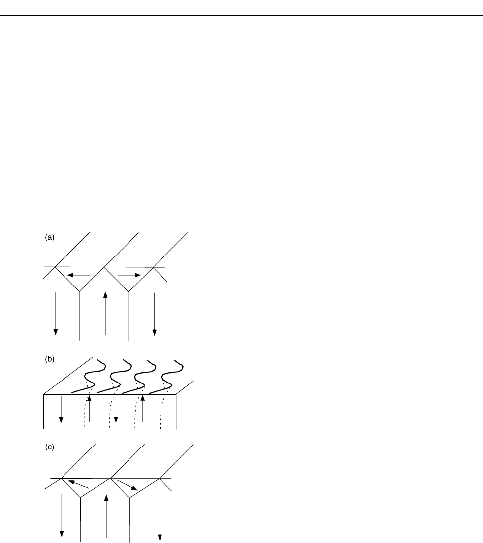
Domains and domain wal ls at crystal surfaces

In relatively thick crystals, domains and domain walls may change

their geometric styles near and at crystal surfaces, in order to lower

the total magnetostatic energy with respect to that of the “open” struc-

ture shown in Figure M14. The particular style depends largely on the

dominant kind of anisotropy, as well as on the relative strengths of

magnetostatic and anisotropy energies. When 2pM

/K  1 in a uniax-

ial material, prism-shaped closure domains bounded by 90



walls, in

which spins rotate through 90



from one domain to the next, may com-

pletely close off magnetic flux at the crystal surface. Lamellar domains

separated by 180



walls may fill the crystal’s volume (Figure M16a).

In this case, the two main energies originate from the walls and from

magnetoelastic energy due to magnetostrictive strain where closure

domains abut body domains. Closure domain structures such as these

can subdivide further into elaborate arrays of smaller closure and

nested spike domains, if the crystal is sufficiently thick. Because clo-

sure domains can either greatly reduce or completely eliminate magne-

tostatic energy, the body domains can be several times broader than

predicted for the Kittel-like, “open” structure.

When 2pM

/K  1 in a uniaxial substance like barium ferrite, a

large amount of anisotropy energy results when M

is perpendicular

to the “easy” axis. Therefore, the style of surface closure shown in

Figure M16a is energetically unfavorable. Instead, a very different

style of surface domain structure may evolve in thick crystals. Walls

which are planar within the body of the crystal can become wavy at

the surface (Figure M16b). In extremely thick crystals, wavy walls

can alternate with rows of reverse spikes. These elaborate surface

domain structures lower magnetostatic energy by achieving a closer

mixture of “positive” and “negative” free magnetic poles (e.g., see

Szymczak, 1968).

Large crystals governed by cubic magnetocrystalline anisotropy

reduce surface flux through prism-shaped closure domains at the sur-

face. When <100> are easy directions, as in iron, closure domains

are bounded by 90



walls (Figure M16a). When <111> are easy

directions, as in magnetite, closure domains are bounded by 71



and

109



walls and, within the closure domains, M

is canted with respect

to the crystal surface (Figure M16c).

Temperature dependence of domain structure

Understanding how domain structure evolves during both heating to

and cooling from the Curie point is crucial to understanding the acqui-

sition and thermal stability of thermal remanent magnetization (TRM).

If the number of domains changes significantly during cooling from

the Curie point, it is reasonable to hypothesize that TRM will not

become blocked until the overall domain structure reaches a stable

configuration.

According to Kittel’s original model (Figure M14), grains will

nucleate (add) domain walls and domains with heating in zero field,

if the wall energy drops more rapidly with increasing temperature than

does the magnetostatic term. Energywise, in this first case a particle

can “afford” to add domains with heating. Conversely, during cooling

from the Curie point a grain will denucleate (lose) domain s and

domain walls if wall energy rises more quickly than does M

with

decreasing temperature. If wall energy drops less rapidly with increas-

ing temperature than does M

, then the opposite scenarios apply. Of

course, such behavior relies on the assumptions that the particle is able

to maintain a global energy minimum (GEM) domain state at all tem-

peratures and that the total magnetostatic energy of the walls them-

selves can be ignored.

Using Amar’s (1958) model, Moskowitz and Halgedahl (1987) cal-

culated the number of domains between room temperature and the

Curie point in parallelepipeds of TM60. As discussed earlier, they

investigated two cases: dominant crystalline anisotropy (zero stress)

and high stress (s ¼ 100 MPa). Magnetostatic energy from wall

moments was included in the calculations. At all temperatures they

assumed that particles occupied GEM domain states. Because the tem-

perature dependences of the material constants A (exchange constant)

and l (magnetostriction constant) for TM60 had not been constrained

well by experiments, they ran six models to bracket the least rapid and

most rapid drops in wall energy with heating.

In TM60 grains larger than a few micrometers, most of their results

gave an increase in the number of domains with heating. Exceptions to

this overall pattern were cases in which walls broadened so dramati-

cally with increasing temperature that they nearly filled the particle

and rendered nucleation unfavorable. During cooling from the Curie

point in zero field, the domain “blocking temperature”—that is,

the temperature below which the number of domain s remained

constant—increased both with decreasing grain size and with internal

stress.

Figure M16 Three styles in which domains and domain walls may

terminate at a crystal surface. (a) Illustration of prism-shaped

surface closure domains at the surface of a material which is either

uniaxial, with 2pM

/K  1.0, or cubic, such as iron, whose easy

axes are along <100>. Here, 90



walls separate closure domains

from the principal “body” domains that fill most of the crystal.

Arrows indicate the sense of spontaneous magnetization within the

domains. (b) Illustration of wavy walls at the surface of a uniaxial

material with 2pM

/K < 1.0. Waviness dies out with increasing

distance from the surface. (c) Prism-shaped closure domains at the

surface of a cubic material, such as magnetite, whose easy

directions of magnetization are along <111>. Closure domains

and body domains are separated by 71



and 109



walls.

MAGNETIC DOMAINS 493

Micromagnetic models

In contrast to classical models of magnetic domain structure, micro-

magnetic models do not assume the presence of discrete domains—

that is, relatively large volumes in a crystal where the spontaneous

magnetization points in a single direction. Instead, micromagnetic

models allow the orientations of M

-vectors to vary among extremely

small subvolumes, into which a grain is divided. A stable configura-

tion is obtained numerically when the sum of exchange, anisotropy,

and magnetostatic energies is minimum. To reduce computation time,

all micromagnetic models for magnetite run to date assume unstressed,

defect-free crystals.

Moon and Merrill (1984, 1985) were the first in rock magnetism to

construct one-dimensional (1D) micromagnetic models for defect-free

magnetite cubes. To simplify calculations, they assumed that magnetite

was uniaxial. In their models, they subdivided a cube into K thin, rec-

tangular lamellae. Within a Kth lamella, the spin vectors were parallel

to the lamella’s largest surface but oriented at angle y

with respect to

the easy axis of anisotropy. The distribution of angles was varied

throughout the cube until a state of minimum energy was obtained.

Because the y

’s varied continuously across the grain, there was no

sharp demarcation between domains and domain walls. For practical

purposes, a wall’s effective width was defined as the region in which

the moments rotated most rapidly. Nucleation was modeled by

“marching” a fresh wall from a particle’s edge into the interior. A

nucleation barrier was determined by calculating the maximum rise

of total energy as the wall moved to its final location and as preexist-

ing walls adjusted their positions to accommodate the new wall. The

denucleation barrier was determined by reversing the nucleation

process.

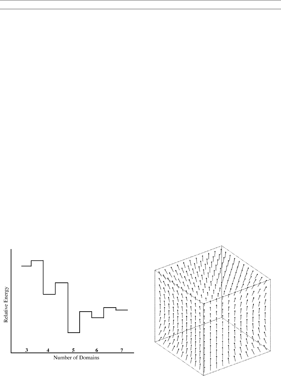
Moon and Merill’s major breakthrough was the discovery that a

particle can occupy a range of local energy minimum (LEM)

domain states. Each LEM state is characterized by a unique number

of domains and is separated from adjacent states by energy barriers.

As illustrated in Figure M17, the GEM state is the configuration of

lowest energy but, owing to the energy barriers between states, a

LEM state can be quite stable as well. Any given LEM can be stable

over a broad range of grain sizes.

Several authors have extended micromagnetic calculations for

magnetite to two- and three-dimensions (e.g., Williams and Dunlop,

1989, 1990; Newell et al., 1993; Xu et al., 1994; Fabian et al., 1996;

Fukuma and Dunlop, 1998; Williams and Wright, 1998). In 2D

models, grains are subdivided into rods. In 3D models, the crystal

is subdivided into a multiplicity of extremely small, cubic cells (e.g.,

 0.01 mm on a side), within each of which M

represents the average

magnetization over several hundred atomic dipole moments. Each

cell’s M

-vector is oriented at angle y with respect to the easy axis,

and the y ’s are varied independently with respect to their neighbors

until an energy minimum is achieved. Owing to the extremely large

number of cells and the even larger number of computations,

energy calculations begin with an initial guess of how the final,

minimum energy structure might appear. To date, the largest mag-

netite cubes addressed by 3D models are only a few micrometers

in size, due to limitations of computing time (e.g., Williams and

Wright, 1998).

2D and 3D micromagnetic models yield a variety of exotic, nonuni-

form configurations of magnetization, such as “flower” and “vortex”

states. Analogous to Moon and Merrill’s results, these models yield

both LEM and GEM states, although very different in their

-structures from those of 1D models. For example, Figure M18

illustrates a “flower” state in a cube magnetized parallel to the z-axis.

The flower state is reminiscent of a classical SD state of uniform

magnetization, except that the M

-vectors are canted at and near

the crystal surface. Increasing the cube size makes other nonuniform

states energetically favorable (e.g., Fabian et al., 1996). For example,

according to 3D models of magnetite cubes between 0.01 and 1.0 mm

in size, the flower state is the lowest energy state between about

0.05 and 0.07 mm (Williams and Wright, 1998). Further increase of

cube size yields a vortex state, in which the M

-vectors circulate

around a closed loop within the grain. By Williams and Wright’scalcula-

tions, both flower and vortex states are stable between about 0.07 and

0.22 mm, although the vortex state has the lower energy. Raising

the cube size to the 0.22–1.0 mm range results in the flower state

becoming unstable, so that the vortex state is the only possible state.

In relatively large cubes of magnetite—e.g., 4 or 5 mm—2D and

3D models yield M

-configurations closely approaching those of

Figure M18 Illustration of a “flower” state obtained through

three-dimensional micromagnetic modeling of a cube largely

magnetized along the cube’s z-axis.

Figure M17 Diagram illustrating the relative energies and energy

barriers associated with local energy minimum (LEM) domain

states. Each LEM state is characterized by a unique number of

domains and is separated from adjacent states by nucleation and

denucleation energy barriers. In this diagram, the global energy

minimum, or GEM, domain state has five domains.

494 MAGNETIC DOMAINS

classical domain structures expected for magnetite; some models predict

“body” domains separated by domain walls, with closure domains at the

surface (e.g., Xu et al., 1994; Williams and Wright, 1998).

According to several micromagnetic models of hysteresis in submi-

cron magnetite, magnetization reversal can occur through LEM-LEM

transitions (e.g., flower to vortex state). Reversal can take place

through almost independent reversals of the particle’s core and outer

shell (e.g., Williams and Dunlop, 1995).

Dunlop et al. (1994) used 1D micromagnetic models to investi-

gate transdomain TRM. Transdomain TRM—that is, acquisition of

TRM through LEM-LEM transitions —had been proposed earlier by

Halgedahl (1991), who observed denucleation of walls and domains

in titanomagnetite during cooling (see below for a discussion of these

results). In particular, Halgedahl’s observations strongly suggested that

denucleation could give rise to SD-like TRMs in grains that, after

other magnetic treatments, contained domain walls. Furthermore,

Halgedahl (1991) found that a grain could “arrive” in a range of

LEM states after replicate TRM acquisitions.

To determine whether transdomain TRM could be acquired by

stress-free, submicron magnetite particles free of defects, Dunlop

et al. (1994) calculated the energy barriers for all combinations among

single domain-two-domain-three-domain transitions with decreasing

temperatures from the Curie point of magnetite in a weak external

field. They assumed that LEM-LEM transitions were driven by ther-

mal fluctuations across LEM-LEM energy barriers and that thermal-

equilibrium populations of LEM states were governed by Boltzmann

statistics. According to their results, after acquiring TRM most popula-

tions would be overwhelmingly biased toward GEM domain states,

and an individual particle should not exhibit a range of LEM states

after several identical TRM runs.

Using renormalization group theory, Ye and Merrill (1995) arrived

at a very different conclusion. According to their calculations, short-

range ordering of spins just below the Curie point could give rise to

a variety of LEM states in the same particle after replicate coolings.

These conflicting theoretical results are discussed below in the

context of experiments.

Domain observations

Methods of imaging domains and domain walls

Rock magnetists have mainly used three methods to image domains

and domain walls: the Bitter pattern method, the magneto-optical Kerr

effect (MOKE), and magnetic force microscopy (MFM). Two other

methods—transmission electron microscopy (TEM) and off-axis elec-

tron holography—have been used in a very limited number of studies

on magnetite.

The Bitter method images domain walls through application of a

magnetic colloid to a smooth, polished surface carefully prepared to

eliminate residual strain from grinding (e.g., see details in Halgedahl

and Fuller, 1983). Colloid particles are attracted by the magnetic field

gradients around walls, giving rise to Bitter patterns. When viewed

under reflected light, patterns appear as dark lines against a grain’s

bright, polished surface. With liquid colloid, this method can re-

solve details as small as about 1 mm. If colloid is dried on the sample

surface and the resultant pattern is viewed in a scanning electron

microscope (SEM), features as small as a few tenths of one micrometer

can be resolved (Moskowitz et al., 1988; Soffel et al., 1990).

The MOKE is based on the rotation of the polarization plane of inci-

dent light by the magnetization at a grain’s surface. Unlike the Bitter

method, the MOKE images domains themselves, rather than domain

walls. Domains appear as areas of dark and light, the result of their

contrasting magnetic polarities (Hoffmann et al., 1987; Worm et al.,

1991; Heider and Hoffmann, 1992; Ambatiello et al., 1999). The

MOKE has the same resolving power as the Bitter method.

In the MFM, a magnetized, needle-shaped tip is vibrated above the

highly polished surface of a magnetic sample. Voltage is induced in the

tip by the magnetic force gradients resulting from domains and domain

walls. The effects of any surface topography are removed by scanning

the surface with the nonmagnetic tip of an atomic force microscope.

The MFM can resolve magnetic features as small as 0.01 mm

(Williams et al., 1992; Proksch et al., 1994; Moloni et al., 1996;

Pokhil and Moskowitz, 1996, 1997; Frandson et al., 2004).

Styles of domains observe d in magnetic minerals of

paleomagnetic significance

In rock magnetism, the majority of domain observation studies have

focused on four magnetic minerals, all important to paleomagnetism:

pyrrhotite (Fe

), titanomagnetite of roughly intermediate composi-

tion (near Fe

2.4

, or TM60), magnetite (Fe

), and hematite

(Fe

Owing to its high magnetocrystalline anisotropy constant and rela-

tively weak magnetostriction constant, pyrrhotite behaves magnetically

as a uniaxial material. When studied with the Bitter method, pyr-

rhotite often exhibits fairly simple domain patterns, which suggest

lamellar domains separated by 180



walls (Figure M19a) (Soffel,

1977; Halgedahl and Fuller, 1983).

Despite being cubic, intermediate titanomagnetites rarely, if ever,

exhibit the arrays of closure domains, 71



, and 109



walls that

one would predict. Instead, these minerals usually display very com-

plex patterns of densely spaced, curved walls. Possibly, these complex

structures result from varying amounts of strain within the particle

(Appel and Soffel, 1984, 1985). Occasionally, grains exhibit simple

arrays of parallel walls, such as that shown in Figure M20 (e.g.,

Halgedahl and Fuller, 1980, 1981), but it is not unusual to observe

wavy walls alternating with rows of reverse spikes (Halgedahl, 1987;

Moskowitz et al., 1988). Both simple and wavy patterns suggest a

dominant, internal stress that yields a uniaxial anisotropy, although

the origin of this stress is still unclear. On one hand, it could originate

from the mechanical polishing required to prepare samples for domain

studies. Alternatively, in igneous rock samples stress could be gener-

ated during cooling, due to differences in the coefficients of thermal

expansion among the various minerals.

Small magnetite grains randomly dispersed in a rock or a synthetic

rock-like matrix generally display simple arrays of straight domain

walls, if the domains’ magnetizations are sufficiently close to being

parallel to the surface of view (e.g., Worm et al., 1991; Geiß et al.,

1996) (Figure M21 ). In such samples, however, there appears to be a

paucity of closure domains, perhaps the result of observation surfaces

being other than {100} planes.

In an early study by Bogdanov and Vlasov (1965), Bitter patterns of



and 109



walls were observed on cleavage planes of a few small

magnetite particles obtained by crushing a natural crystal. Similarly,

from Bitter patterns Boyd et al. (1984) found both closure domains

and networks of 180



,71



, and 109



walls in several magnetite parti-

cles in a granodiorite. Body domains accompanied by closure domains

were also reported by Smith (1980), who applied the TEM method to a

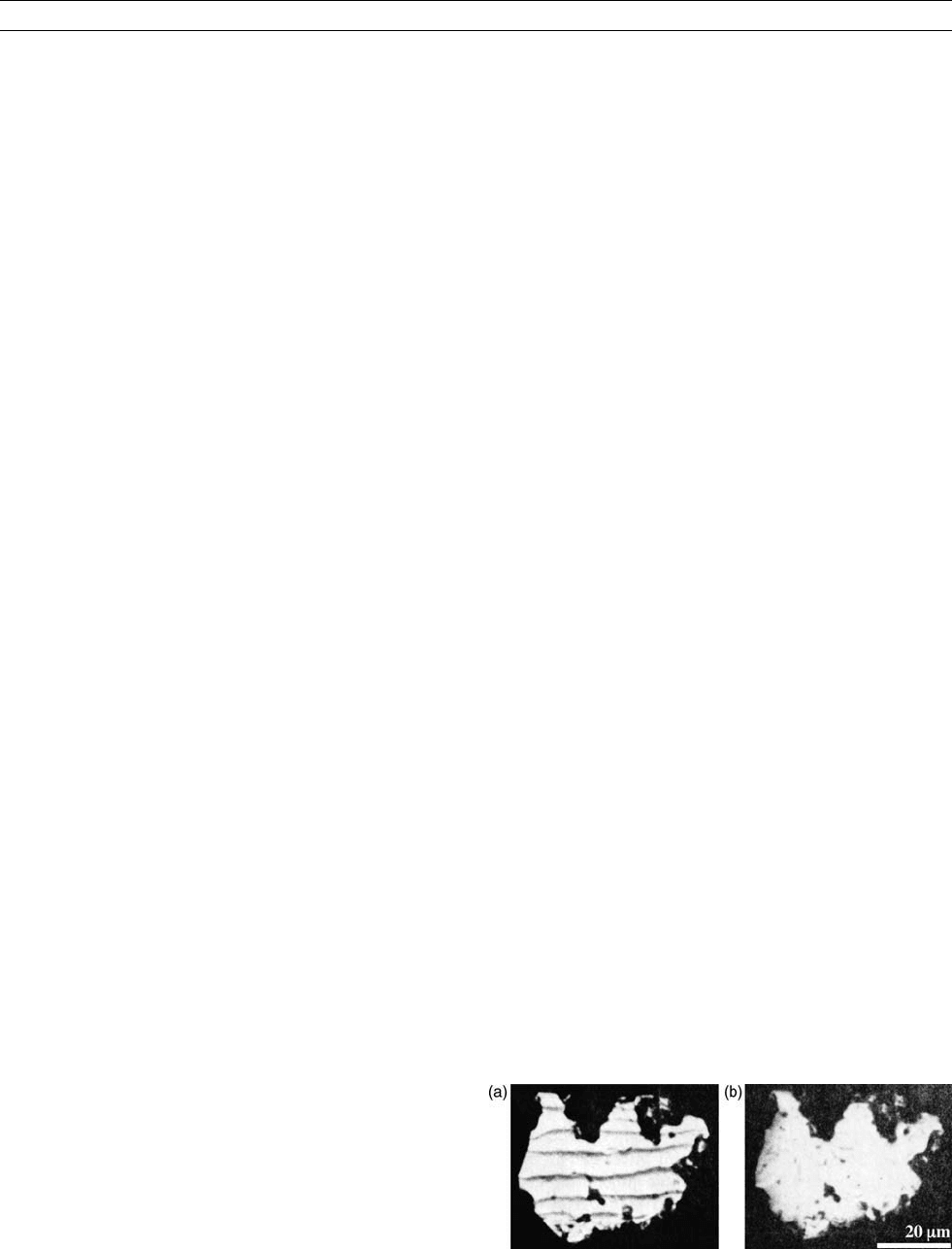
Figure M19 Bitter patterns on a particle of natural pyrrhotite

(a) after demagnetization in an alternating field of 1000 Oe and (b)

in an apparently SD-like state after acquiring saturation

remanence in 15 kOe.

MAGNETIC DOMAINS 495