Keyfitz N., Caswell H. Applied Mathematical Demography

Подождите немного. Документ загружается.

13.1. Eigenvalue Sensitivity 305

13.1 Eigenvalue Sensitivity

13.1.1 Perturbations of Matrix Elements

We begin with the sensitivity of an eigenvalue λ to changes in the ma-

trix elements a

. The functional dependence of λ on the a

is expressed

implicitly in the characteristic equation

det(A − λI)=0.

When the form of the characteristic equation is known, implicit diﬀerenti-

ation can be used to ﬁnd ∂λ/∂a

(Hamilton 1966, Demetrius 1969, Emlen

1970, Goodman 1971, Keyﬁtz 1971a, Mertz 1971a). We will use this ap-

proach in Section 13.1.6, but it is limited to cases in which the characteristic

equation is suﬃciently simple that implicit diﬀerentiation yields a simple

solution.

A general approach, applicable to matrices of any structure, was intro-

duced by Caswell (1978). The formula dates back at least to Jacobi (1846),

and has been rediscovered many times (e.g., Faddeev 1959, Faddeev and

Faddeeva 1963, Desoer 1967). For a complete and rigorous discussion, see

Kato (1982). Cohen (1978, p. 186) presents an alternative approach to

eigenvalue sensitivity.

We begin with the equations deﬁning the eigenvalues and the right and

left eigenvectors:

= λ

(13.1.1)

∗

A = λ

∗

, (13.1.2)

where v

∗

is the complex conjugate transpose of v

. For the moment, let

us suppress the subscript i; the following formulae apply to any of the

eigenvalues and their corresponding right and left eigenvectors. Taking the

diﬀerential of both sides of (13.1.1) yields

A(dw)+(dA)w = λ(dw)+(dλ)w, (13.1.3)

where dA =(da

) is a matrix whose elements are the diﬀerentials da

Form the scalar product

∗

of both sides with the left eigenvector v,

A(dw), v + (dA)w, v = λ(dw), v + (dλ)w, v. (13.1.4)

Expanding the scalar products and cancelling terms leaves

dλ =

(dA)w, v

w, v

(13.1.5)

∗

dAw

∗

. (13.1.6)

∗

The scalar product of the vectors x and y is x, y = y

∗

306 13. Perturbation Analysis of Matrix Models

Suppose that only one element, a

, is changed, while all the others are

held constant. Then dA contains only one nonzero entry, da

,inrowi and

column j, and (13.1.6) reduces to

dλ =

¯v

w, v

, (13.1.7)

where ¯v

is the complex conjugate of v

. Dividing both sides by da

and

rewriting the diﬀerentials as partial derivatives (since all but one of the

variables of which λ is a function are being held constant), we get the

formula

†

∂λ

∂a

¯v

w, v

. (13.1.8)

That is, the sensitivity of λ to changes in a

is proportional to the

product of the ith element of the reproductive value vector and the jth

element of the stable stage distribution. The scalar product term in the

denominator is independent of i and j, and can be ignored when considering

the relative sensitivities of λ to diﬀerent elements in the same matrix. Or,

the eigenvectors may be scaled so that w, v = 1, so that the term can be

ignored.

It is easy to calculate a sensitivity matrix S whose entries give the

sensitivities of λ to the corresponding entries of A:

S =



∂λ

∂a



(13.1.9)

w, v

. (13.1.10)

The sensitivity is the local slope of λ, considered as a function of a

13.1.2 Sensitivity and Age

The sensitivity of λ to changes in age-speciﬁc survival and fertility plays

an important role in the theory of senescence (Medawar 1952, Williams

1957, Hamilton 1966, Rose 1984, Wachter and Finch 1997, Carey 2003).

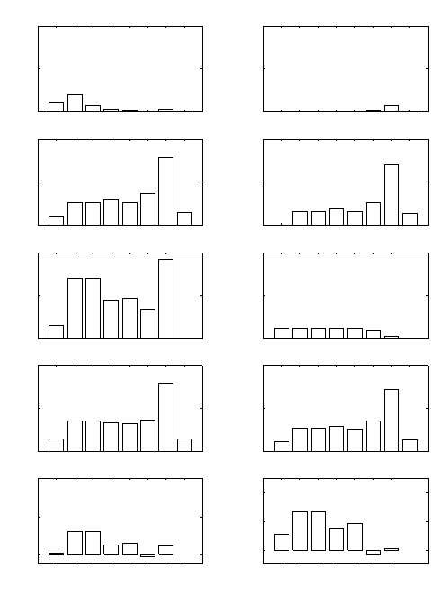
Figure 13.1 shows these sensitivities for four populations (a ﬂour beetle,

a vole, a whale, and humans). Sensitivities of λ to fertility decline nearly

exponentially with age. At early ages, λ is more sensitive to changes in

survival than to changes in fertility. At older ages, the pattern is reversed.

The sensitivities vary by as much as eight orders of magnitude.

†

This formula is often written with v

in place of ¯v

. This makes no diﬀerence in the

analysis of λ

, since v

is real, but could cause errors in computing sensitivities of other

eigenvalues, and of eigenvectors.

13.1. Eigenvalue Sensitivity 307

0 10 20

−8

−7

−6

−5

−4

−3

−2

−1

Age

Sensitivity of λ

C. oryzae

0 10 20

Age

M. orcadensis

0 25 50

Age

O. orca

0 25 50

Age

H. sapiens

Figure 13.1. The sensitivity of λ to changes in age-speciﬁc fertility F

and survival

probability P

for (from left to right) a laboratory population of the ﬂour beetle

Calandra oryzae (Birch 1948), a laboratory population of the vole Microtus orca-

densis (Leslie et al. 1955), the killer whale Orcinus orca (Olesiuk et al. 1990), and

the human population of the United States in 1965 (Keyﬁtz and Flieger 1968).

Some of these properties can be derived directly from the sensitivity

formula. The eigenvectors w and v for age-classiﬁed populations are

= 1 (13.1.11)

= P

···P

i−1

−i+1

for i>1, (13.1.12)

and

= 1 (13.1.13)

= F

−1

+ P

−1

i+1

for i>1. (13.1.14)

We can use w and v to show how the sensitivities change with age

(Demetrius 1969, Caswell 1978, 1982c). From (13.1.8) and (13.1.12) it

follows that

∂λ/∂F

j+1

(13.1.15)

. (13.1.16)

Thus the sensitivity of λ to fertility is a strictly decreasing function of

age as long as λ>1. If the P

are constant, then the decrease will be

308 13. Perturbation Analysis of Matrix Models

exponential, as is approximately true in Figure 13.1. Other things being

equal, the sensitivity of λ to changes in fertility falls oﬀ with age more

rapidly the greater the value of λ. In a decreasing population, however, the

sensitivity will actually increase from age j to j +1ifλ<P

The sensitivities of λ to changes in survival at successive ages satisfy

∂λ/∂P

j+1

j+2

(13.1.17)



j+1

−1

+ P

j+1

j+2



(13.1.18)

= λ

j+1

j+2

(13.1.19)

≥

j+1

if λ ≥ 1. (13.1.20)

Thus the sensitivity of λ to survival decreases monotonically with age pro-

vided λ ≥ 1andP

j+1

≥ P

. If survival were age-independent, then the

sensitivity of λ to changes in survival would decrease monotonically with

age provided λ>1.

The relative sensitivities of λ to fertility and survival satisfy

∂λ/∂P

∂λ/∂F

j+1

(13.1.21)

j+1

. (13.1.22)

Thus λ is more sensitive to survival than to fertility if v

j+1

,whichis

true at least up to the age of ﬁrst reproduction. In Figure 13.1, ∂λ/∂P

∂λ/∂F

for young ages; the inequality is reversed at older ages.

13.1.3 Sensitivities in Stage- and Size-Classiﬁed Models

The patterns of sensitivity in size- or stage-classiﬁed models can be quite

diﬀerent from those in age-classiﬁed models. Because the stable size distri-

bution may exhibit peaks (as is commonly observed in ﬁsh and tree size

distributions), sensitivities need not be monotonic functions of size or stage.

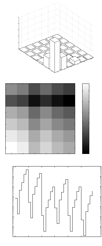
Example 13.1 Size-speciﬁc sensitivity in the desert tortoise

Figure 13.2 shows the sensitivity of λ to changes in the F

, P

,and

. None of the sensitivities shows a monotonic trend with size. Pop-

ulation growth rate is very sensitive to changes in the vital rates of

size classes 2 and 3, and also size class 7.

Example 13.2 Sensitivity analysis of teasel

In stage-classiﬁed models, there may be no variable, like size, against

which sensitivities can be plotted. In this case, it is useful to display

13.1. Eigenvalue Sensitivity 309

0 1 2 3 4 5 6 7 8 9

0.2

0.4

Sensitivity of λ ...

to F

1 2 3 4 5 6 7 8

0.2

0.4

to P

1 2 3 4 5 6 7

0.2

0.4

to G

1 2 3 4 5 6 7 8

0.2

0.4

to σ

0 1 2 3 4 5 6 7 8 9

0.2

0.4

to γ

Size class i

0 1 2 3 4 5 6 7 8 9

0.2

0.4

Elasticity of λ ...

1 2 3 4 5 6 7 8

0.2

0.4

1 2 3 4 5 6 7

0.2

0.4

1 2 3 4 5 6 7 8

0.2

0.4

1 2 3 4 5 6 7

0.02

0.04

Size class i

Figure 13.2. Perturbation analysis of population growth rate for the desert tor-

toise. Left column shows sensitivities, right column elasticities, of λ to F

, P

, G

, and γ

. Calculated from data of Doak et al. (1994), medium-high fertility.

the entire sensitivity matrix S calculated from (13.1.10):

S =

⎛

⎜

⎝

0.067 0.028 0.001 0.007 0.001 0.001

0.002 0.001 0.000 0.000 0.000 0.000

0.421 0.174 0.008 0.046 0.008 0.003

2.442 1.011 0.046 0.265 0.047 0.018

16.432 6.801 0.313 1.786 0.315 0.119

47.475 19.650 0.905 5.160 0.911 0.344

⎞

⎟

⎠

. (13.1.23)

310 13. Perturbation Analysis of Matrix Models

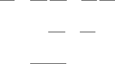
The matrix can be displayed graphically as a surface plot or an image

plot, or by plotting the entries of vec S (Figure 13.3).

‡

These plots

all show that λ is most sensitive to changes in entries in the lower-

left corner of the matrix. These entries correspond to growth directly

from seeds to large rosettes and ﬂowering plants. Such growth doesn’t

happen in this species (i.e., these entries of A are all zero), but that

does not change the fact that if those probabilities were changed, the

impact on λ would be considerable.

13.1.4 What About Those Zeros?

The sensitivity (13.1.7) gives the eﬀect on λ of changes in any entry of A,

including those that may, in a given context, be regarded as ﬁxed at zero or

some other value. This is exactly as it should be. The derivative tells what

would happen to λ if a

were to change, not whether, or in what direction,

or how much, a

actually changes (Caswell et al. 2000). The results of

such impossible perturbations may or may not be of interest, but they are

not zero. It is up to you to decide whether they are useful and whether to

display them.

For example, in the projection matrix for teasel, a

= 0 because ﬂow-

ering plants neither survive nor produce new ﬂowering plants in one year.

But from the sensitivity matrix (13.1.23) we see that

∂λ

∂a

=0.344.

If a

were changed by a small amount ∆a

, the resulting change in λ

would be approximately 0.344∆a

. This bit of information would be of

no interest to someone concerned with environmental perturbations, but

very interesting indeed to someone studying the evolution of annual and

biennial life histories.

13.1.5 Total Derivatives and Multiple Perturbations

The sensitivity (13.1.8) is written as the partial derivative of λ with respect

to a

, holding all other parameters constant. If more than one parameter

is perturbed simultaneously, the net eﬀect on λ is given by the diﬀerential

dλ =



k,l

∂λ

∂a

. (13.1.24)

This result can be used in several ways.

‡

The vec operator produces a vector from a matrix by stacking the columns one

above the other.

13.1. Eigenvalue Sensitivity 311

Sensitivity of λ

Log

sensitivity of λ

−4

−3

−2

−1

1 2 3 4 5 6

−5

−4

−3

−2

−1

Column

Sensitivity of λ

Figure 13.3. Three ways of displaying the sensitivity matrix S for teasel (Field

A). The upper graph plots sensitivities as a surface, the middle graph as an

image, and the lower graph as a plot of vec S. In the lower graph, the numbers

are coordinates (i, j) of the entry of S.

312 13. Perturbation Analysis of Matrix Models

1. Lower-level parameters. Suppose that one or more of the matrix

entries are functions a

(x) of some “lower-level” variable x (e.g.,

allocation of energy to reproduction, which aﬀects both survival and

fertility). Then

∂a

∂x

dx. (13.1.25)

Substituting this expression into (13.1.24) yields the chain rule

dλ



k,l

∂λ

∂a

∂x

(13.1.26)

2. Physiological or genetic constraints. One vital rate may be function-

ally related to another, for many reasons. Increased fertility may

result in decreased somatic growth, because of allocation of resources.

Increased survival early in life may result in decreased survival later

in life due to pleiotropic eﬀects. We suppose that perturbing one vital

rate a

will aﬀect some or all of the other matrix entries, so that

∂a

. (13.1.27)

Substituting into (13.1.24), we obtain

dλ

∂λ

∂a



kl=ij

∂λ

∂a

. (13.1.28)

3. A special case of constraints arises when individuals face mutually

exclusive options. Consider seeds that may either germinate or remain

dormant. Clearly, P [germination] = 1 − P [dormancy], and a change

in one must produce a compensatory change in the other.

Example 13.3 Sensitivity to survival and growth in size-classiﬁed

models

The parameters G

and P

in the standard size-classiﬁed model for

the desert tortoise are functions of the survival probability (σ

)and

the growth probability (γ

) of size class i. From (13.1.26) we have

∂λ

∂σ

∂λ

∂G

∂σ

∂λ

∂P

∂σ

(13.1.29)

∂λ

∂G

∂λ

∂P

(1 − γ

) (13.1.30)

+ γ

∆v

)

w, v

, (13.1.31)

13.1. Eigenvalue Sensitivity 313

where ∆v

= v

i+1

− v

is the change in reproductive value from size

class i to i + 1. Similarly,

∂λ

∂γ

∂λ

∂G

∂γ

∂λ

∂P

∂γ

(13.1.32)

= σ



∂λ

∂G

−

∂λ

∂P



(13.1.33)

∆v

w, v

. (13.1.34)

The sensitivity of λ to growth rate (13.1.34) is negative if v

i+1

That is, λ is reduced by increasing the growth rate from N

to N

i+1

if stage i + 1 has a lower reproductive value than stage i.

Applying (13.1.31) and (13.1.34) to the size-classiﬁed model for the

desert tortoise yields the results shown in Figure 13.2. This untangles

the survival and growth components of the sensitivities to P

and G

Changes in the survival of stage 7 would have a major impact on

λ. The sensitivity of λ to γ

is slightly negative because of a slight

decline in reproductive value from stage 6 to stage 7.

In the desert tortoise, the fertilities F

were considered independent of

survival and growth. More detailed descriptions of the F

, however, usually

involve both the σ

and γ

. In such cases, the sensitivity of λ to the lower-

level parameters must also include their eﬀects on fertility.

13.1.6 Sensitivity to Changes in Development Rate

Population growth rate is sensitive to changes in the timing of events in

the life cycle (e.g., Lewontin 1965, Mertz 1971, Caswell and Hastings 1980,

Caswell 1982c, Hoogendyk and Estabrook 1984, Ebert 1985). In Section

6.3 we saw the eﬀect on the intrinsic rate of increase r =logλ of changes

in the mean µ and variance σ

of the net maternity function. Increasing µ

corresponds to a delay in development, and an analysis using age-classiﬁed

matrices yields the same conclusion as (6.3.5); i.e., that in an increasing

population, delayed reproduction reduces population growth rate.

However, this analysis is based on the transformation of the charac-

teristic equation into a cumulant generating function, and holds only for

age-classiﬁed models. What can we say about slowing the rate of transition

in a general stage-classiﬁed model?

To answer this question, we start with a transformation of a life cycle

graph (Section 9.1.3). The coeﬃcient on each arrow is multiplied by λ

−α

where α is the number of projection intervals required for the transition.

Once transformed, the graph can be simpliﬁed by multiplying the coeﬃ-

cients on pathways between any two stages (see MPM Chapter 7). Figure

13.4 shows such a graph, focusing on the transition from stage j to stage

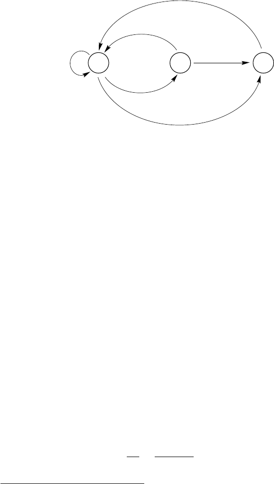
314 13. Perturbation Analysis of Matrix Models

(λ)

−α

Figure 13.4. A life cycle graph for evaluating the sensitivity of λ to changes in α,

the time required for the transition from stage j to stage i.

i, which requires α projection intervals to complete, with a probability P

of surviving. The other arcs in this graph represent

• a(λ) for all paths between N

and N

that do not pass through N

• b(λ) for all paths between N

and N

that do not pass through N

• c(λ) for all paths between N

and N

• d(λ) for all paths from N

to N

which do not pass through N

• e(λ) all loops involving neither N

nor N

We assume that there are no disjoint loops in the graph. The following

method can be extended to life cycles containing such loops, but the results

are more complicated. Since the time (α) required for transition from N

to N

appears explicitly in the transformed life cycle graph, it is possible to

evaluate the sensitivity of λ to changes in development rate between these

two stages.

The characteristic equation can be written down from the graph

1=a(λ)c(λ)Pλ

−α

+Φ(λ) (13.1.35)

= F(λ), (13.1.36)

where Φ(λ)=a(λ)b(λ)+c(λ)d(λ)+e(λ). Implicit diﬀerentiation of λ with

respect to α gives

∂λ

∂α

−∂F/∂α

∂F/∂λ

. (13.1.37)

By setting equal to 1 the product of the transmissions around all loops in the graph;

see MPM Chapter 7.