Keyfitz N., Caswell H. Applied Mathematical Demography

Подождите немного. Документ загружается.

13.4. Comparative Studies and Life Table Response Experiments 325

VITAL

RATES

POPULATION

STATISTICS

POPULATION

STATISTICS

(1)

VITAL

RATES

(N)

SYNTHESIS

ANALYSIS

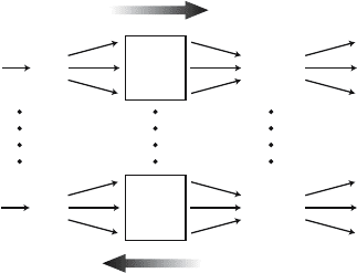
Figure 13.9. The design of a LTRE. Treatments (T

–T

) produce environmental

conditions (E

–E

) that aﬀect all the various vital rates. The vital rates are

collected into population projection matrices A

(1)

–A

(N)

, from which a variety of

population statistics can be calculated. From Caswell (1996a).

or fertility at a given age increases relative reproductive value at

earlier ages, and decreases it at later ages.

13.4 Comparative Studies and Life Table Response

Experiments

It is often of interest to compare the demography of two or more popula-

tions. Biologists often do so by imposing experimental manipulations and

measuring the resulting vital rates. Because of this, the methods of this

chapter are called life table response experiments (LTREs), but even in bi-

ological applications the word “experiment” must be understood broadly,

including not only designed manipulative experiments but also compara-

tive observations. It is still useful to think in terms of experiments, but to

recognize that the treatments may be applied by nature rather than by the

investigator.

In a LTRE, a life table (or more generally a set of vital rates) is the

response variable in an experimental design or comparative study (Caswell

1989a, 1996a,b, 2000b). Treatments modify the environment and change the

vital rates of individuals (Figure 13.9). The eﬀects on the vital rates are

usually diverse (aﬀecting survival and reproduction and growth, sometimes

in diﬀerent directions) and stage-speciﬁc. Demographic models synthesize

these eﬀects into statistics that quantify the treatment eﬀects at the popu-

lation level. Population growth rate λ is the most frequently used statistic

and the one focused on here, but others can be used.

326 13. Perturbation Analysis of Matrix Models

The ﬁrst true LTRE was Birch’s (1953) study of the eﬀects of tempera-

ture, moisture, and food on three species of ﬂour beetles. The approach has

become widely used in studies of chronic exposure to toxic substances; see

Levin et al. (1996) for a recent example and van Straalen and Kammenga

(1998) for a review with additional references.

The relation between λ and treatment shows how the treatments aﬀect

population growth, but it obscures the cause of those eﬀects. Suppose that λ

has been reduced; is it because mortality was increased, or growth impaired,

or reproduction limited? Are these causes all equally responsible for the

eﬀect on λ, or can parts of that eﬀect be attributed to each of them?

To answer these questions requires a decomposition of the treatment

eﬀect on λ into contributions from each stage-speciﬁc vital rate. This

decomposition pinpoints the vital rates responsible for the population

level eﬀect of the treatment. It was introduced by Caswell (1989); several

methodological extensions have appeared since (Brault and Caswell 1993,

Caswell 1996a,b, 2000b). Applications include Levin et al. (1987, 1996),

Levin and Huggett (1990), Walls et al. (1991), Silva et al. (1991), Canales

et al. (1994), Brault and Caswell (1993), Caswell and Kaye (2001), Hansen

(1997), Horvitz et al. (1997), and Ripley (1998).

LTREs can be classiﬁed by their design, in analogy to analysis of

variance:

1. Fixed designs: the treatments imposed (by the experimenter or by

nature) are of interest in themselves. Examples might include levels

of toxicant exposure or food supply.

(a) One-way designs: comparison of two or more levels of a single

treatment factor.

(b) Factorial designs: two or more levels of each of two or more

treatment factors applied in all possible combinations.

2. Random designs: The treatments are a random sample from some

distribution of treatment levels. Examples might include quadrats

randomly distributed within a region (thereby sampling microhabi-

tat variability), or a sequence of years (randomly sampling climatic

conditions). It is often diﬃcult to decide if a factor is ﬁxed or random.

One way to decide is to ask if you would use the same levels if you

were to repeat the experiment. The answer is probably yes in the case

of toxicant levels in a laboratory bioassay (a ﬁxed factor) and no in

the case of quadrats randomly located within the forest (a random

factor). Random designs come in one-way, factorial, and nested vari-

eties; some of these are only beginning to be explored (Caswell and

Dixoninprep.).

3. Regression designs: The treatments represent levels of some quantita-

tive factor (e.g., concentration of pesticide), and the goal is to explore

the functional dependence of λ on the factor.

13.5. Fixed Designs 327

Notation alert. We use superscripts in parentheses to denote treat-

ments, and subscripts to denote matrix elements. Thus A

(i)

is the

projection matrix obtained under treatment i, λ

(i)

is its dominant eigen-

value, and a

(i)

the (k, l)entryofA

(i)

. Means are denoted by replacing a

superscript by a dot; e.g.,

(·)



(j)

, (13.4.1)

where m is the number of levels of the treatment.

13.5 Fixed Designs

The approach to a ﬁxed design LTRE is to write a linear model for λ as

a function of the treatments, and use the sensitivities of λ to obtain the

coeﬃcients in the linear model.

13.5.1 One-Way Designs

Consider a one-way design with treatments T

,...,T

producing popu-

lation growth rates λ

(1)

,...,λ

(N)

.Chooseareference matrix A

(r)

as a

baseline against which to measure treatment eﬀects. A

(r)

might be the

mean matrix A

(·)



(i)

, or the matrix for a particular level of the

treatment, often a “control.”

Expanding λ, as a function of the a

, around A

(r)

gives the population

growth rate in treatment m as

(m)

≈ λ

(r)



i,j



(m)

− a

(r)



∂λ

∂a



†

m =1,...,N, (13.5.1)

where

†



(m)

+ A

(r)



/2. (13.5.2)

The terms in the summation in (13.5.1) are the contributions of the a

the eﬀect of treatment m on population growth.

The sensitivities in (13.5.1) are evaluated at a matrix A

†

which is “mid-

way” between the two matrices, A

(m)

and A

(r)

, being compared. This is

not absolutely essential, and other matrices, such as A

(m)

or A

(r)

,could

be used instead. However, using A

†

includes some information on the cur-

vature of λ as a function of the a

. The mean value theorem of calculus

guarantees that, for each treatment m, there is a matrix somewhere between

(m)

and A

(r)

that will make the approximation (13.5.1) exact. Since it is

halfway between, A

†

has a good chance of being close to this matrix. Using

†

has been shown to give good results, and Logofet and Lesnaya (1997)

have shown that it provides, in a sense, the best approximation.

328 13. Perturbation Analysis of Matrix Models

0 10 20 30 40

0.2

0.4

0.6

0.8

Age

Survivorship

Planktotrophic

Lecithotrophic

0 10 20 30 40

100

150

Age class

Fertility

Planktotrophic

Lecithotrophic

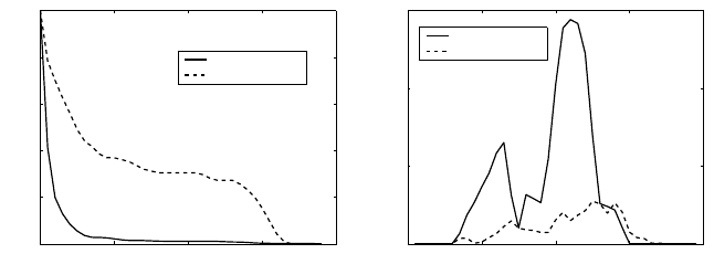
Figure 13.10. Survivorship and fertility for the planktotrophic and lecithotrophic

strains of the polychaete Streblospio benedicti. From Levin et al. (1987).

These calculations can easily be implemented by deﬁning a matrix of

diﬀerences

(m)

= A

(m)

− A

(r)

m =1,...,N

and then calculating a matrix of contributions as

(m)

= D

(m)

◦ S

†

, (13.5.3)

where ◦ is the Hadamard (element-by-element) product.

Example 13.8 Larval development mode in Streblospio benedicti

Streblospio benedicti is a marine polycheate worm that is capable

of explosive population growth. It reproduces by a planktonic lar-

val stage. Two genetic strains exist; in one the larvae are equipped

with yolk and do not feed (lecithotrophic larvae), in the other the

larvae are not provisioned with yolk, and must feed in the plankton

(planktotrophic larvae); see Levin et al. (1987). Because they invest

so much more in each oﬀspring, the lecithotrophic strain has lower

fertility, but the oﬀspring have higher survival probability (Figure

13.10). We want to know how these life history diﬀerences contribute

to diﬀerences in λ.

In laboratory experiments, Levin et al. (1987) measured projection

matrices A

(l)

for lecithotrophs and A

(p)

for planktotrophs, with rates

of increase λ

(l)

=1.319 and λ

(p)

=1.205.

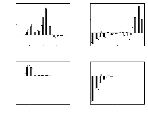
We choose the lecithotrophic matrix A

(l)

as the reference matrix. Fig-

ure 13.11 shows the diﬀerences in age-speciﬁc fertility F

and survival

probability P

; the planktonic strain has a huge fertility advantage,

especially from ages 15–25, and a survival disadvantage early in life.

However, the large fertility diﬀerences between 20 and 30 weeks of

age make almost no contribution to the diﬀerence in λ.Indeed,all

but a very small proportion of the eﬀect on λ is contributed by fertil-

ity and survival eﬀects occurring before 15 weeks of age. Adding the

13.6. Random Designs and Variance Decomposition 329

0 10 20 30 40

−50

100

150

Difference

0 10 20 30 40

−0.08

−0.04

0.04

Contribution

Age

0 10 20 30 40

−0.5

0.5

Difference

0 10 20 30 40

−0.08

−0.04

0.04

Age

Contribution

Figure 13.11. (Top row) The diﬀerences in age-speciﬁc fertility (F

) and survival

) between the planktotrophic and lecithotrophic strains of Streblospio bene-

dicti. (Bottom row) The contributions of those diﬀerences to the eﬀect of larval

development mode on λ.

fertility contributions (which total 0.1710) and the survival contribu-

tions (which total −0.3315) shows that, while the survival diﬀerences

appear less dramatic than the fertility diﬀerences, they actually

contribute more to the eﬀect on λ. This analysis quantiﬁes the intu-

itive notion of a “trade-oﬀ” between increased fertility and reduced

survival in comparison of larval development modes.

Even though developmental mode has large eﬀects on the vital rates

and on λ in this experiment, the ﬁrst-order approximation in (13.5.1)

is very accurate. It predicts

(p)

= λ

(l)



i,j

=1.1590,

where c

is the contribution of a

. This is within 4 percent of the

actual value of λ

(p)

13.6 Random Designs and Variance Decomposition

In a random design, the results are characterized by the variance in λ,and

the goal of the analysis is to decompose this variance into contributions

from the variances in (and covariances among) the matrix entries (Brault

and Caswell 1993, Horvitz et al. 1997).

330 13. Perturbation Analysis of Matrix Models

Let V (λ) denote the variance in λ among treatments. To ﬁrst order, V (λ)

can be written

V (λ) ≈



C(ij, kl)s

, (13.6.1)

where C(ij, kl) is the covariance of a

and a

, and the sensitivities s

and s

are evaluated at the mean matrix. Each term in the summation is

the contribution of one vital rate covariance to V (λ). Unless there is good

reason to believe that the vital rates are independent, the covariance terms

in this calculation should not be neglected.

Suppose that there are n stages, and that the mean matrix is

A.The

contributions can be calculated easily by deﬁning a n

× n

covariance

matrix

C = E



vec (A)vec (A)



− vec (

A)vec (

(13.6.2)

and then computing a n

× n

matrix of contributions

V = C ◦



vec (S)vec (S)



. (13.6.3)

Contributions to V (λ) can also be calculated in terms of lower-level pa-

rameters. Suppose that the a

are deﬁned in terms of stage-speciﬁc growth

probabilities γ

, survival probabilities σ

, and reproductive outputs m

,for

i =1,...,n. Deﬁne a parameter vector

p =(σ

, ···,σ

,γ

, ···,γ

n−1

, ···,m

) .

In terms of p,thevarianceV (λ)is

V (λ) ≈



Cov (p

)

∂λ

∂p

∂λ

∂p

, (13.6.4)

where the sensitivities are evaluated by applying (13.1.26) to the matrix

calculated from the mean of the parameters.

Example 13.9 Interpod variance in λ in killer whales

Killer whales (Orcinus orca) live in stable social groups called pods.

Brault and Caswell (1993) developed stage-classiﬁed models for each

of the 18 pods of resident killer whales in the coastal waters of Wash-

ington state and British Columbia (Examples 9.1 and 11.1). The

model (Figure 3.10) included four stages: yearlings, juvenile females,

mature females, and senescent females, with a projection matrix

A =

⎛

⎜

⎝

0 F

0 G

00G

⎞

⎟

⎠

Pod-speciﬁc population growth rates ranged from λ =0.9949 to λ =

1.0498, with a variance V (λ)=2.90 × 10

−4

13.6. Random Designs and Variance Decomposition 331

−1

x 10

−3

(d)

Covariances

(c)

(b)

(a)

−1

x 10

−4

(d)

Contributions to V(λ)

(c)

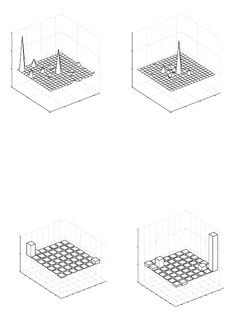
Figure 13.12. (Left) The interpod covariances of the matrix entries a

for the

killer whale. (Right) The contributions of the covariances to V (λ). The matrix

entries are listed in the order produced by vec (A). Letters identify the most

conspicuous peaks: (a) variance in G

, (b) covariance of G

and G

, (c) variance

in P

, and (d) variance in F

. From data of Brault and Caswell (1993).

−0.01

0.01

Covariances

−1

x 10

−4

Contributions to V(λ)

Figure 13.13. The covariances among the lower-level parameters and their contri-

butions to V (λ) for killer whales. Parameters 1–4 are σ

–σ

, 5–6 are γ

–γ

, and

7ism. Calculated from data of Brault and Caswell (1993).

Figure 13.12 shows the covariance matrix C and the contribution ma-

trix V for this population. The largest variance is that of G

(yearling

survival), but this makes no detectable contribution to V (λ). The

largest contribution to V (λ)isfromvarianceinF

(adult fertility).

ThereisalargecovariancebetweenG

and G

, but it makes almost

no contribution to V (λ).

Using the lower-level parameters

p =

(γ

does not appear because it is always 1) gives a clearer picture

of the determinants of V (λ). Figure 13.13 shows the covariances

among these parameters and their contributions to V (λ). The largest

contributions come from V (m), V (σ

), and V (γ

), in that order.

332 13. Perturbation Analysis of Matrix Models

0 1 2 3 4 5 6 7 8

−1

−0.5

0.5

1.5

Concentration (x)

Concentration effect dλ/dx

Growth rate λ

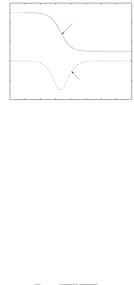
Figure 13.14. A hypothetical example showing λ as a function of concentration

(x) and the eﬀect of x, measured as the rate of change of λ with respect to x.

13.7 Regression Designs

The goal of a regression design is to describe the response of λ to the level

of some quantitative factor x. In an ordinary linear regression analysis,

the “eﬀect” of the independent variable x on the dependent variable y is

measured by the slope of the regression line. Accordingly, we deﬁne the

eﬀect of x on λ as the slope ∂λ/∂x. Unless λ is a linear function of x (and

there is no reason to expect that it will be) the slope will vary with x. Figure

13.14 shows a hypothetical example, in which λ is measured as a function

of the concentration x of some substance. The substance has little eﬀect

at low concentrations, large negative eﬀects at intermediate concentrations

(from x =2tox = 4), and little or no eﬀect at high concentrations. This

intuitive interpretation is captured by using the slope of the function as

the measure of eﬀect.

The data for a regression LTRE consist of a set of vital rates a

(x)that

are functions of the treatment variable x. These vital rates generate a set

of matrices A

(x)

and population growth rates λ(x). The eﬀect of x on λ

can be decomposed into contributions from each of the vital rates using

the chain rule

dλ



i,j

∂λ

∂a

(x)

∂a

(x)

∂x

. (13.7.1)

This expression is exact, not an approximation. The derivatives ∂λ/∂a

(x)

are calculated from the matrix A

(x)

. The vital rate sensitivity ∂a

(x)/∂x

comes from the functional relationship between the vital rates and x.This

13.8. Prospective and Retrospective Analyses 333

relationship can be described in various ways: interpolation of observed val-

ues, ﬁtting parametric relationships (linear or nonlinear), or nonparametric

smoothing (Caswell 1996a).

The terms in the summation in (13.7.1) are the contributions of each

of the vital rates to the treatment eﬀect on λ at a speciﬁc value of x.

The contribution can be positive or negative, depending on the sign of

∂a

(x)/∂x. The contribution of a

(x)willbesmallifa

(x)isnotvery

sensitive to x,orifλ is not very sensitive to a

(x), or both.

These contributions can be summed in various ways, to describe the con-

tributions of diﬀerent groups of vital rates. Summing over all fertilities, for

example, would give an integrated contribution of eﬀects on reproduction:



∂λ

∂F

(x)

∂F

(x)

∂x

. (13.7.2)

Summing the contributions of all the a

gives an approximation to the

derivative of λ with respect to x. Integrating this derivative then gives an

estimate of λ(x) that can be compared with the observed response to see

how well the functions a

(x) capture the response of the vital rates to x.

For an example of this analysis applied to a toxicological experiment, see

Caswell (1996a).

13.8 Prospective and Retrospective Analyses

This chapter has avoided discussing the “importance” of the vital rates,

because the term admits two meanings. The a

might be considered “im-

portant” because s

or e

were large, and hence if a

were to be perturbed,

λ would change a lot. On the other hand, a

might be considered “impor-

tant” because the variability in λ is determined more by variability in a

than by variability in any other rate.

These two deﬁnitions are not—nor should they be expected to be—

equivalent, and are distinguished as “prospective” and “retrospective”

perturbation analysis (Caswell 1997, Horvitz et al. 1997, Caswell 2000a).

Prospective analysis looks forward, and asks what will happen if a

is per-

turbed. Sensitivity and elasticity analysis provide the answer. Retrospective

analysis looks back at some observed set of matrices A

and asks how much

the (co)variance of the a

contributed to the variance in λ. LTRE analysis,

in its various guises, is the appropriate tool.

Prospective analysis is independent of any pattern of variation; indeed, it

will happily and correctly give the results of changes in the vital rates that

are biologically impossible (“What if this annual plant became a perennial;

What if this plant without seed dormancy began to have some; What if

pigs could ﬂy . . . ”). Retrospective analysis, in contrast, is speciﬁc to the

observed variation in the vital rates. The contribution of the variance in

334 13. Perturbation Analysis of Matrix Models

to V (λ) can be low either because λ is insensitive to a

or because a

happened not to vary much in the set of observations at hand, or both.

The distinction is particularly important in conservation, where (over-

simplifying a bit) managers want to increase λ by imposing some policy,

and they want to do so eﬃciently and economically. All else being equal,

the best choice is a policy that targets those vital rates with highest sen-

sitivity or elasticity; the proper tool is prospective sensitivity analysis. For

a more detailed discussion, see MPM, Chapter 18.