Kline R.B. Principles and Practice of Structural Equation Modeling

Подождите немного. Документ загружается.

24 CONCEPTS AND TOOLS

violations of this requirement may not be critical, but more serious ones can result in

bias. This bias can affect not only the regression weights of predictors measured with

error but also those of other predictors. However, it is difﬁcult to anticipate the direc-

tion of this error propagation. Depending on sample intercorrelations, some regression

weights may be biased upward (too large), but others may be biased in the other direc-

tion. There is no requirement that the criterion should be measured without error, but

the use of a psychometrically inadequate measure of it can reduce the value of R

. When

the predictors are measured without error but the criterion is measured with error, beta

weights tend to be too small, but not the unstandardized regression weights. If the pre-

dictors are measured with error, too, then these effects for the criterion could be ampli-

ﬁed, diminished, or canceled out, but it is best not to hope for the latter. See Liu (1988)

for more information.

4. It is assumed that omitted predictors are uncorrelated with measured predictors,

or those in the equation. This requirement is a consequence of the fact that the residuals

are uncorrelated with the predictors in OLS estimation. This is a strong assumption, one

that is probably violated in most applications of MR (and SEM, too). This assumption

also concerns the issue of speciﬁcation error, which is considered next.

speciﬁcation error

Speciﬁcation error refers to the problem of omitted predictors that account for some

unique proportion of total criterion variance but are not included in the analysis. A

related term is left-out-variable error or, more lightheartedly, the “heartbreak of

L.O.V.E.” The idea of speciﬁcation error in SEM is even broader than in MR, but the

omission of relevant predictors is a concern in SEM, too. Suppose that r

= .40 and r

.60 for, respectively, predictors X

and X

. A researcher measures only X

and uses it as

the sole predictor of Y. The standardized regression coefﬁcient for the included predictor

in this bivariate analysis is r

= .40. If the researcher had the foresight to also measure

, the omitted predictor, and enter it along with X

as a predictor in an MR analysis, the

beta weight for X

in this analysis may not equal .40. If not, then r

as a standardized

regression coefﬁcient with X

as the sole predictor does not reﬂect the true predictive

power of X

compared with b

derived with both predictors in the equation. However,

the difference between r

and b

varies with r

, the correlation between the included

and omitted predictors. Speciﬁcally, if the included and omitted predictors are unrelated

taBle 2.1. example data set for Multiple regression

Case X

3 65 24

8 50 20

10 40 22

15 70 32

19 75 27

Fundamental Concepts 25

= 0), there is no difference (r

= b

) because there is no correction for correlated

predictors. But as the absolute value of their correlation increases (r

≠ 0), the amount

of the difference between r

and b

due to the omission of X

becomes greater.

Presented in Table 2.2 are the results of three pairs of regression analyses. In all

pairs, X

is considered the omitted predictor.

One member of each pair of analyses is a

bivariate regression with X

as the sole predictor, and the other member is an MR with

both X

and X

in the equation. Constant across all three sets of analyses are the bivari-

ate correlations between the predictors and the criterion (r

= .40, r

= .60). The only

thing that varies across the three sets is the value of r

, the correlation between the pre-

dictors. Reported for each analysis in Table 2.2 are the standardized regression weights

for the bivariate regression; b

and b

for the MR) and also the overall multiple

correlation (

12Y

⋅

) for the regression of Y on both X

and X

. For each case in the table,

compare in the same row the value of r

in boldface with that of b

, also in boldface.

The difference between these values (if any) indicates the amount by which the bivariate

standardized regression coefﬁcient for X

does not accurately reﬂect its predictive power

relative to when X

is also in the equation.

Note in Table 2.2 that when the omitted predictor X

is uncorrelated with the

included predictor X

(case 1, r

= 0), the standardized regression weight for X

is the

same regardless of whether or not X

is in the equation (r

= b

= .40). However, when

= .30 (case 2), the value of b

is lower than that of r

, respectively, .24 versus .40.

This happens because b

controls for the correlation between X

and X

, whereas r

does not. Thus, r

overestimates the association between X

and Y relative to b

. In

case 3 in the table, the correlation between the included and omitted predictors is even

higher (r

= .60), which for these data results in an even greater discrepancy between

and b

(respectively, .40 vs. .06).

Omitting a predictor correlated with others in the equation does not always result

in overestimation of the predictive power of an included predictor. For example, if X

the included predictor and X

is the omitted predictor, it is also possible for the absolute

value of r

to be less than that of b

(i.e., r

underestimates the relation indicated by b

)

The same principles hold if X

is the omitted predictor and X

is the included predictor.

taBle 2.2. examples of the omitted variable Problem

Predictor(s)

Both X

and X

Case X

only X

Y ⋅ 12

1. r

= 0 .40 .40 .60 .72

2. r

= .30 .40 .24 .53 .64

3. r

= .60 .40 .06 .56 .60

Note. Numerical values for X

and X

are standardized regression coefﬁcients.

For all cases, X

is considered the omitted variable; r

= .40 and r

= .60.

26 CONCEPTS AND TOOLS

or even for r

and b

to have different signs. Both cases indicate suppression. However,

overestimation due to omission of a predictor probably occurs more often than under-

estimation (suppression). Also, the pattern of bias may be more complicated when there

are several included and omitted variables (e.g., overestimation for some included pre-

dictors; underestimation for others).

Predictors are typically excluded because they are not measured. Thus, it is difﬁcult

to know by how much and in what direction regression coefﬁcients may be biased rela-

tive to what their values would be if all relevant predictors were included. However, it

is unrealistic to expect the researcher to know and be able to measure all relevant pre-

dictors. In this way, all regression equations are probably misspeciﬁed to some degree.

If omitted predictors are uncorrelated with included predictors, the consequences of

speciﬁcation error may be slight. Otherwise, the consequences may be more serious.

Careful review of theory and research is the main way to avoid a serious speciﬁcation

error by decreasing the potential number of left-out variables.

suppression

Perhaps the most general deﬁnition is that suppression occurs when either the absolute

value of a predictor’s beta weight is greater than its bivariate (zero-order) correlation

with the criterion or the two have different signs. So deﬁned, suppression implies that

the estimated relation between a predictor and a criterion while controlling for the other

predictors is a “surprise,” given the bivariate correlations. Suppose that X

is amount of

psychotherapy, X

is degree of depression, and Y is number of prior suicide attempts.

The bivariate correlations in a hypothetical sample are

= .19, r

= .49, and r

= .70

Based on these results, it may seem that psychotherapy is harmful because of its posi-

tive association with suicide attempts (r

= .19). When both predictors (depression,

psychotherapy) are entered as predictors in the same regression equation, however, the

results are

= –.30, b

= .70, and

12Y

⋅

= .54

The beta weight for psychotherapy (–.30) has the opposite sign of its bivariate correla-

tion with the criterion (.19), and the beta weight for depression (.70) exceeds its bivariate

correlation (.49).

The “surprising” results just described are due to controlling for other predic-

tors. Here, people who are more depressed are also more likely to be in psychotherapy

= .70). Depressed people are more likely to try to harm themselves (r

= .49).

Corrections for these associations in MR reveal that the relation of psychotherapy to

suicide attempts is actually negative once depression is controlled. It is also true that

the relation of depression to suicide attempts is even stronger once psychotherapy is

Fundamental Concepts 27

controlled. Omit either psychotherapy or depression from the analysis—a speciﬁcation

error—and the bivariate regression results with the remaining predictor are mislead-

ing. This example concerns negative suppression, where the predictors have positive

correlations with the criterion and each other, but one receives a negative beta weight

in the analysis.

A second type of suppression is classical suppression, where one predictor is uncor-

related with the criterion but receives a nonzero beta weight controlling for another pre-

dictor. For example, given the following correlations in a hypothetical sample,

= 0, r

= .60, and r

= .50

the results of an MR analysis are

= –.40, b

= .80,

12Y

⋅

= .69

This example of classical suppression (i.e., r

= 0, b

= –.40) demonstrates that bivari-

ate correlations of zero can mask true predictive relations once other variables are con-

trolled. There is also reciprocal suppression, which can occur when two predictors

correlate positively with the criterion but negatively with each other. See Shieh (2006)

for more information about suppression.

death to stepwise regression, think for Yourself

There are two basic ways to enter predictors into the equation: One is to enter all pre-

dictors at once, or simultaneous entry. The other is to enter predictors over a series of

steps, or sequential entry. Entry order can be determined according to one of two dif-

ferent standards, theoretical (rational) or empirical (statistical). The rational standard

corresponds to hierarchical regression, where you tell the computer a ﬁxed order of

entry for the predictors. For example, sometimes demographic variables are entered at

the ﬁrst step, and then entered at the second step is a psychological variable of interest.

This order not only controls for the demographic variables but also permits evaluation

of the predictive power of the psychological variable, over and beyond that of simple

demographic variables.

An example of the statistical standard is stepwise regression, where the com-

puter selects predictors for entry based on statistical signiﬁcance (e.g., which predictor,

if entered into the equation, would have the most statistically signiﬁcant regression

weight?). After they are selected, predictors at a later step can also be removed from the

equation according to statistical test outcomes (e.g., if a predictor’s regression weight is

no longer statistically signiﬁcant). The stepwise process stops when there could be no

statistically signiﬁcant increase in R

by adding more predictors. There are variations

on stepwise regression—for example, some methods select predictors but do not later

remove them (forward inclusion), and others begin with all predictors in the equation

and then automatically remove them (backward elimination)—but all such methods

are directed by the computer, not you.

28 CONCEPTS AND TOOLS

Stepwise regression and related methods pose many problems, so many that such

methods are now basically forbidden in some research areas (e.g., Thompson, 1995), and

for good reason, too. One problem is extreme capitalization on chance. Another is that

not all regression computer programs print correct values of statistical tests in stepwise

regression; that is, the computer’s choices may actually be wrong. Both of these prob-

lems imply that whatever ﬁnal set of predictors happen to be selected by the computer

in empirically driven procedures is unlikely to replicate. Worst of all, such methods give

the illusion that the researcher does not have to think about the problem. Sribney (1998)

offers this advice: “Personally, I would no more let an automatic routine select my model

than I would let some best-ﬁt procedure pack my suitcase” (Ronan Conroy’s Comments

section, para. 8).

In SEM, there are methods for modifying structural equation models with poor ﬁt

to the data that are analogous to empirically based methods in MR. These methods in

SEM indicate the particular effects that would result in the greatest improvement in ﬁt

if those effects were added to the model. Some SEM computer tools, such as LISREL,

offer an automatic modiﬁcation (AM) option that mechanically adds effects according

to statistical criteria. Such purely exploratory options greatly capitalize on chance; they

also give the illusion that you need not think about the problem. I do not recommend

the use of AM-type options. Instead, the modiﬁcation of your model should be guided

mainly by your hypotheses, just as its speciﬁcation in the ﬁrst place should be so guided.

There is a role in SEM for more limited empirically based methods, but they should be

used in a way that respects your hypotheses. These issues are elaborated in Chapter 8,

on hypothesis testing in SEM.

PartIal CorrelatIon and Part CorrelatIon

The technique of partial correlation concerns the phenomenon of spuriousness: if the

observed relation between two variables is due to ≥ 1 common cause(s), their association

is spurious. To illustrate this concept, consider these zero-order correlations between

vocabulary breadth (Y), shoe size (X

), and age (X

) in a hypothetical sample of children

not all the same age:

= .50, r

= .60, and r

= .80

Although the correlation between shoe size and vocabulary breadth is fairly substantial

(.50), it is hardly surprising because both are caused by a third variable, age (i.e., matu-

ration).

The partial correlation

12Y

⋅

removes the inﬂuence of a third variable X

from both

and Y. The formula is

1 2 12

2 12

( 1 ) ( 1 )

rrr

⋅

−

−−

(2.10)

Fundamental Concepts 29

The denominator in Equation 2.10 adjusts the total standardized variance of both Y and

for their overlap with X

. Applied to the hypothetical correlations just listed, the

partial correlation between shoe size and vocabulary breadth controlling for age is

12Y

⋅

= .04. (An exercise will ask you to calculate this partial correlation.) Because the asso-

ciation between X

and Y essentially disappears when X

is controlled, their observed

relation r

= .50 may be a spurious one. The technique of SEM readily allows the repre-

sentation of presumed spurious associations due to common causes.

Equation 2.10 for partial correlation can be extended to control for two or more

external variables. For example, the higher-order partial correlation

1 23Y

⋅

estimates

the association between X

and Y controlling for both X

and X

. There is a related

coefﬁcient called part correlation or semipartial correlation that partials external

variables out of either of two variables, but not both. The formula for the part correlation

( 1 2 )Y

⋅

for which the association between X

and X

is controlled but not the association

between Y and X

is presented next:

1 2 12

(1 2 )

rrr

⋅

−

(2.11)

Note that the denominator in Equation 2.11 adjusts the total standardized variance only

for the overlap of X

with X

. Given the same bivariate correlations among these three

variables reported earlier, the part correlation between vocabulary breadth (Y) and shoe

size (X

) controlling only the latter for age (X

) is

( 1 2 )Y

⋅

= .03. This result (.03) is some-

what smaller than the partial correlation for these data, or

12Y

⋅

= .04. In general,

12Y

⋅

is larger in absolute value than

( 1 2 )Y

⋅

. An exception is when r

= 0; in this case,

12Y

⋅

( 1 2 )Y

⋅

Relations among the squares of the various correlations just described can be nicely

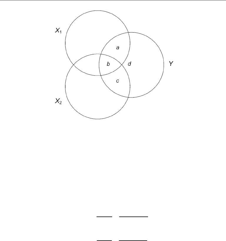
illustrated with a Venn-type diagram like the one in Figure 2.1. The circles represent the

total standardized variances of the criterion Y and the predictors X

and X

. The regions

in the ﬁgure labeled a–d make up the total standardized variance of Y, so

a + b + c + d = 1.0

Areas a and c in the ﬁgure represent the portions of Y uniquely predicted by, respectively,

and X

, but area b represents the simultaneous overlap (redundancy) of the predictors

with Y. Area d represents the proportion of unexplained variance. The squared zero-

order correlations of the predictors with the criterion and the overall squared multiple

correlation can be expressed as sums of the areas a, b, c, or d in Figure 2.1, as follows:

= a + b and

= b + c

12Y

⋅

= a + b + c = 1.0 – d

The squared part correlations correspond directly to the unique areas a and c in Fig-

ure 2.1. Each of these areas also equals the increase in the total proportion of explained

variance that occurs by adding a second predictor to the equation. That is,

30 CONCEPTS AND TOOLS

222

(1 2 ) 12 2YYY

raRr

⋅⋅

==−

(2.12)

222

( 2 1) 12 1YYY

rcRr

⋅⋅

==−

In contrast, the squared partial correlations correspond to areas a, c, and d in Figure 2.1,

and each estimates the proportion of variance in the criterion explained by one predic-

tor but not the other. The formulas are

12 2

ad r

⋅

−

+−

(2.13)

12 1

cd r

⋅

−

+−

Note that the numerator of each expression in Equation 2.13 is a squared part correla-

tion. The denominators in Equation 2.13 correct the total standardized variance of the

criterion for its overlap with the other predictor. These denominators are generally < 1.0,

which explains why squared partial correlations are generally larger than squared part

correlations. Suppose that

12Y

⋅

= .40 and

= .25. These results follow:

( 1 2 )Y

⋅

= .40 – .25 = .15

12Y

⋅

= .15/(1 – .25) = .20

In words, predictor X

uniquely explains .15, or 15% of the total variance of Y (squared

part correlation). Of the variance in Y not already explained by X

, predictor X

accounts

FIgure 2.1. Venn diagram for the standardized variances of Y, X

, and X

Fundamental Concepts 31

for .20, or 20% of the remaining variance (squared partial correlation). See G. Garson

(2009) for an online review of partial correlation and part correlation.

When predictors are correlated—which is just about always—beta weights, par-

tial correlations, and part correlations are alternative ways to describe in standardized

terms the relative explanatory power of each predictor controlling for the rest. None is

more “correct” than the other because each gives a different perspective on the same

data. However, remember that unstandardized regression coefﬁcients (B) are preferred

when comparing results for the same predictors across different samples.

other BIvarIate CorrelatIons

When all observed variables are continuous, it is Pearson correlations that are usually

analyzed in SEM as part of analyzing covariances. (Recall that cov

is the product of

and the standard deviations of each variable; Equation 1.1.) However, noncontinu-

ous variables can be analyzed in SEM, too, so you need to know something about other

kinds of bivariate correlations. There are other forms of the Pearson correlation for

observed variables that are either categorical or ordinal. For example:

1. The point-biserial correlation (r

) is a special case of r that estimates the

association between a dichotomous variable and a continuous one (e.g., gender,

weight).

2. The phi coefﬁcient (

) is a special case for two dichotomous variables (e.g.,

treatment-control, relapsed-not relapsed).

3. Spearman’s rank order correlation or Spearman’s rho is for two ranked vari-

ables.

It is also possible in SEM to analyze non-Pearson correlations that assume the under-

lying data (i.e., on a latent variable) are continuous and normally distributed instead of

discrete. For example:

1. The biserial correlation is for a continuous variable and a dichotomy (e.g.,

agree-disagree), and it estimates what the Pearson r would be if both variables

were continuous and normally distributed.

2. The polyserial correlation is the generalization of the biserial correlation that

does basically the same thing for a continuous variable and a categorical vari-

able with three or more levels.

3. The tetrachoric correlation for two dichotomous variables estimates what r

would be if both variables were continuous and normally distributed.

http://faculty.chass.ncsu.edu/garson/PA765/partialr.htm

32 CONCEPTS AND TOOLS

4. The polychoric correlation is the generalization of the tetrachoric correlation

that estimates r but for categorical variables with two or more levels.

Computing polyserial or polychoric correlations is complicated (Nunnally & Bernstein,

1994) and requires specialized software such as PRELIS, which is the part of LISREL for

manipulating, generating, and transforming data. The PRELIS program can be used to

estimate polyserial or polychoric correlations, depending on the types of variables in the

data set. It can also estimate results for censored variables, which have large propor-

tions of their scores at minimum or maximum values. Consider the variable “price paid

for a new car in the last year.” In a hypothetical sample, only 10% bought a new car year

in the last year, so the scores for rest (90%) are zero. This variable is censored because

not everyone buys a new car every year. Instead of deleting the 90% of the cases who did

not purchase a new car, PRELIS would attempt to estimate results for this variable in the

whole sample assuming that the underlying distribution is normal. Options for analyz-

ing non-Pearson correlations in SEM are considered in Chapter 7.

logIstIC regressIon

Sometimes outcome variables are dichotomous or binary variables. Examples include

graduated–did not graduate and survived–died. Some options to analyze dichotomous

outcomes in SEM are based on the logic of logistic regression (LR). This technique is

generally used instead of MR when the criterion is dichotomous. Just as in MR, the pre-

dictors in LR can be either continuous or categorical. However, the regression equation

in LR is a logistic function that approximates a nonlinear relation between the dichoto-

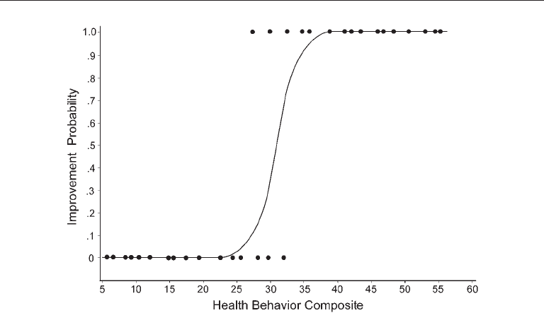
mous outcome and a linear combination of the predictors. An example of a logistic func-

tion for a hypothetical sample is illustrated in Figure 2.2. The closed circles in the ﬁgure

represent along the Y-axis whether cases with the same illness either improved (Y = 1.0)

or did not improve (Y = 0). Along the X-axis, the closed circles in the ﬁgure represent

scores on a composite variable made up of various indexes of healthy behavior (exercise,

preventative care, etc.). The logistic function ﬁtted to the data in Figure 2.2 is S-shaped,

or sigmoidal in form. This function generates predicted probabilities of improvement,

given scores on the healthy behavior composite.

The estimation method in logistic regression is not OLS. Instead, it is usually ML

estimation but is applied after transforming the binary outcome into a logit variable,

which is typically the natural logarithm—base e, or approximately 2.71828—of the

odds of the target outcome. The latter tell us how much more likely it is that a case is a

member of the target group instead of a member of the other group (Wright, 1995), and

it equals the probability of the target outcome divided by the probability of the other

outcome. An example follows.

Suppose that 60% of the cases improved over a particular time, but the rest, or 40%,

did not. Assuming that improvement is the target outcome, the odds of improvement

are calculated here as .60/.40, or 1.5. That is, the odds are 3:2 in favor of improvement.

Fundamental Concepts 33

Regression coefﬁcients for each predictor in LR can be converted into an odds ratio,

which estimates the difference in the odds of the target outcome for a one-point differ-

ence in the predictor, controlling for all other predictors. For example, if the estimated

odds ratio for amount of exercise were 5.60, then the odds of improvement are 5.6 times

greater for each one-point increase on the exercise variable, holding constant other pre-

dictors. Values of odds ratios less than 1.0 would indicate for this example a relative

reduction in the odds of improvement given higher scores on that predictor, and odds

ratios that equal 1.0 would indicate no difference in improvement odds for any value of

the predictor. See Peng, Lee, and Ingersoll (2002) for more information about LR.

statIstICal tests

Characteristics of statistical tests especially relevant for SEM are emphasized next.

standard errors

Perhaps the most basic form of a statistical test is the critical ratio, which is the ratio of

a sample statistic over its standard error. The standard error is the standard deviation

of a sampling distribution, which is a probability distribution of a statistic based on

all possible random samples, each based on the same number of cases. A standard error

estimates sampling error, the difference between sample statistics and the correspond-

ing population parameter. Given constant variability among population cases, standard

FIgure 2.2. Example of a logistic function where closed circles represent actual data values

and the curve represents predicted probabilities.