Korn G.A. Advanced Dynamic-system Simulation: Model-replication Techniques and Monte Carlo Simulation

Подождите немного. Документ загружается.

2 Introduction to Dynamic-system Simulation

Computer simulations can be speeded up or slowed down at the experi-

menter’s convenience. You can simulate a flight to Mars or to Alpha Centauri

in one second. Periodic clock interrupts synchronizing suitably scaled simu-

lations with real time permit “hardware in the loop”: you can “fly” a real

autopilot—or a real human pilot—on a tilting platform controlled by a com-

puter flight simulation. In this book, we are interested in very fast simulation,

for we want to study the effects of many different model changes.

Specifically, we want to

1. Enter and edit programs in convenient editor windows.

2. Use typed or graphical-interface commands to start, stop, and pause

simulations, to select displays, and to make parameter changes. Results

ought to appear immediately to provide an intuitive “feel” for the

effects of model changes (interactive modeling).

3. Program systematic parameter-influence studies and produce cross-

plots or tables.

4. Program model changes to optimize effectiveness measures, and study

effects of random parameter changes or random model inputs by taking

statistics on repeated simulations (Monte Carlo simulation).

1-2. Differential-equation Models

Continuous-system simulation models delayed interactions of physical state

variables

x1, x2, … with first-order ordinary differential equations (state

equations)

(d/dt) xi = fi(t; x1, x2, …; y1, y2, …; a1, a2, …) (i = 1, 2, …) (1-1a)

Here

t represents the time, and the quantities

yj = gj(t; x1, x2, ...; y1, y2, …; b1, b2, …) (j = 1, 2, …) (1-1b)

are defined variables.

a1, a2, …, and b1, b2, … are constant model

parameters.

Simulation programs exercise such models by solving the state-equation

system (1-1) to produce time histories of the system variables

xi = xi(t) and

yj = yj(t) for t = t0 to t = t0 + TMAX, starting with given initial values t0 and

xi(t0). In Section 1-6 and Chapter 2, we shall add sampled-data operations

representing periodic inputs and outputs, sample-holds, and digital

controllers.

The state variables xi are system outputs. They start at t = t0 with given

initial values; subsequent values are produced by an integration routine

(Section 1-7) from the

fi-values generated by the preceding execution

(derivative call) of the operations (1).

There are three kinds of defined variables

yj:

1. system inputs (specified functions of the time

2. system outputs

3. intermediate results needed to compute the derivatives

It must be possible to sort the defined-variable assignments (1-1b) into a pro-

cedure that successively derives all the

yj from state variables xi and/or the

time

t without recurrence relations or “algebraic loops” (Section 1-9).

Some dynamic systems (e.g., systems involving interconnected mechani-

cal devices in automotive engineering and robotics) are modeled with differ-

ential-equation systems that cannot be explicitly solved for state-variable

derivatives as in Eq. (1-1). Simulation then requires solution of algebraic

equations at each integration step. Such differential-algebraic-equation

(DAE) systems are not treated in this book. References [1–4] describe suit-

able mathematical methods and special software.

1-3. Interactive Modeling—Experiment Protocol and

Simulation Studies

Practical computer simulation is not simply a matter of programming and

solving model equations. We must also make it convenient to modify our

models and try many different experiments (see also Section 1-5). In addition

to DYNAMIC program segments listing the model equations (1-1), each sim-

ulation study requires an experiment protocol program that sets and changes

initial conditions and model parameters, calls computer runs, and displays or

tabulates solutions for different model configurations.

The simplest experiment protocols are just sequences of successive

commands, say

a = 20.0 | b = – 3.35 (set parameter values)

x = 12.0 (set the initial value of x)

drun (make a differential-equation

-solving simulation run)

reset (reset initial values)

a = 20.1 (change model parameters)

b = b – 2.2

drun (try another run)

Dynamic-system Models and Computer Programs 3

Each drun command calls a differential-equation-solving simulation run, and

reset resets initial conditions. Typed commands ought to execute immediately

to permit interactive modeling. The operator inspects the solution output after

each simulation run and then types new commands for the next run. Command-

mode operation also permits interactive program debugging [5].

A simulation study combines such commands into a storable program seg-

ment (experiment-protocol script) that can branch and loop to call repeated

simulation runs for different parameter combinations. Simulation studies

may involve thousands of model and parameter changes, so programming

must be easy and computations must be as fast as possible. This is why we

like to interpret experiment-protocol scripts and compile the program seg-

ments executing the actual simulation runs.

1-4. Simulation Software

Commercially available equation-oriented simulation programs such as

ACSL

accept system equations in a more or less human-readable form,

sort defined variable assignments as needed, and feed the sorted equations to

an optimizing Fortran or c compiler [5]. Berkeley Madonna and DESIRE

(see below) have built-in equation-language compilers and execute immedi-

ately. Block-diagram interpreters (e.g., Simulink

, Vissim

, and the open-

source program Scicos) permit graphical block-diagram composition and

immediately execute interpreted simulation runs. Such programs usually pro-

vide equation-language blocks for complicated expressions. Interpreted code

is slow; production runs are sometimes translated into c for faster execution.

Alternatively, ACSL

, Easy5

, and Berkeley Madonna have block-diagram

preprocessors for compiled simulation programs. More advanced modeling

is possible with the Modelica language [6–8].

1-5. OPEN DESIRE and DESIRE

The simulation programs described in this book, and, in particular, our new

techniques for model replication (vectorization), Monte Carlo simulation,

and submodels (Chapters 3–7), use the open-software simulation package

OPEN DESIRE for Linux, Unix including Cygwin (Unix under Windows),

and Microsoft Windows

, or the commercially available DESIRE/2000

program for Windows.

DESIRE simulation systems allow inexpensive per-

sonal computers and workstations solve thousands of differential equations

in seconds.

4 Introduction to Dynamic-system Simulation

The earlier (1995) Windows version of DESIRE discussed in References [1,2] lacks the

vector-compilation features used in this book.

How a Simulation Run Works 5

DESIRE uses double-precision (64-bit) floating-point arithmetic and

accepts command scripts and model descriptions in a readable mathematical

notation such as

y = a

cos(x) + b d/dt x = – x + 4

Command scripts can include operating-system calls, shell scripts, and calls to

other computer programs. DESIRE’s command-script language is itself a

general-purpose mathematical language and handles vectors, matrices, and

even complex numbers (e.g., for frequency-response and root-locus plots) [9].

Programs are entered and edited in editor windows (Fig. 1-1). Each program

begins with an experiment-protocol script that is interpreted much like an

advanced Basic dialect. When the experiment-protocol script encounters a

drun statement, a built-in runtime compiler automatically compiles a

DYNAMIC program segment listing model equations. The state-equation-

solving simulation run then executes at once and produces solution displays

in bright color.

Very fast compilation (typically under 50 ms) simplifies interactive mod-

eling. Experimenters can immediately observe results of programmed or

screen-edited models and experiment-protocol changes. One can enter and

edit different models in multiple editor windows and run these models in turn

to compare results (Fig. 1-1). Runtime displays show solution time histories

and error messages during rather than after each simulation run, so that you

can save time by aborting undesirable runs before they complete.

The experiment-protocol script starting each DESIRE program defines an

experiment. Subsequent DYNAMIC program segments define models used

in the experiment and specify runtime input/output requests. An experiment

protocol can call multiple DYNAMIC segments with different models, dif-

ferent versions of the same model, and/or different input/output operations.

HOW A SIMULATION RUN WORKS

1-6. Sampling the DYNAMIC Segment Variables

When

drun calls a simulation run, the program initializes input/output opera-

tions requested by the DYNAMIC program segment. The independent variable

t (simulation time) and the differential-equation state variables start with initial

values assigned by the experiment protocol.

A first pass through the

DYNAMIC-segment code [Eq. (1-1)] produces initial values of the defined

Unspecified initial values of unsubscripted differential-equation state variables conveniently

default to 0.

6 Introduction to Dynamic-system Simulation

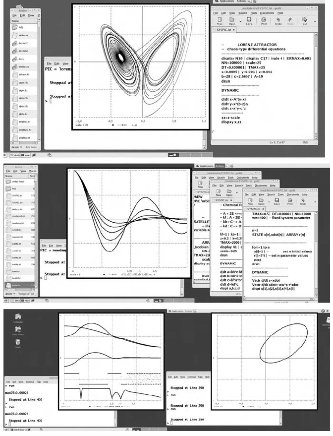
FIGURE 1-1

. OPEN DESIRE running under Linux. The first dual-monitor screen shows a

file-manager window for calling user programs, the DESIRE command window, a graph win-

dow, and an editor window. The second screen has a file manager and three editor windows;

one can click on any file-manager or editor window to run and compare different programs.

On the third screen, two independent simulations run in separate command windows. Solution

graphs were set to black-on-white for publication, but normally each displayed curve has a dif-

ferent color.

How a Simulation Run Works 7

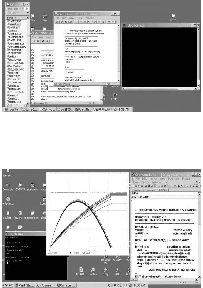
FIGURE 1-1

. DESIRE on a dual Windows

screen showing a file manager window, two

editor windows, and a command Window. The red OK button on each DESIRE editor window

transfers the selected edited program to DESIRE. This makes it convenient to compare two or

more programs.

FIGURE 1-1

. Cygwin (Unix under Windows

) display with a Unix console window, the

DESIRE graphics window, and an editor window using the open-source Crimson Editor. The

original display was in color.

variables [Eq. (1-1b)]. Unless stopped, simulations run from the initial time t =

t0 to t = t0 + TMAX. You can stop a simulation run by typing ctrl c and space

(zz under Windows), and restart or extend a run with drun.

DESIRE normally samples DYNAMIC-segment variables for output (usu-

ally to displays) or sampled-data operations at

NN uniformly spaced sam-

pling times (communication times):

t = t0, t0 + COMINT, t0 + 2 COMINT, … ,

t0 + (NN – 1)COMINT = t0 + TMAX (1-2a)

with

COMINT = TMAX/(NN – 1) (1-2b)

The experiment-protocol script sets appropriate values of

t0, TMAX, and

NN or uses default values listed in the DESIRE manual.

If the DYNAMIC program segment contains differential equations

(d/dt

or Vectr d/dt statements), then t0 defaults to t0 = 0 unless another value is

specified. Starting at

t = t0, the integration routine increments t by successive

constant or variable

DT steps until t reaches the next data-sampling commu-

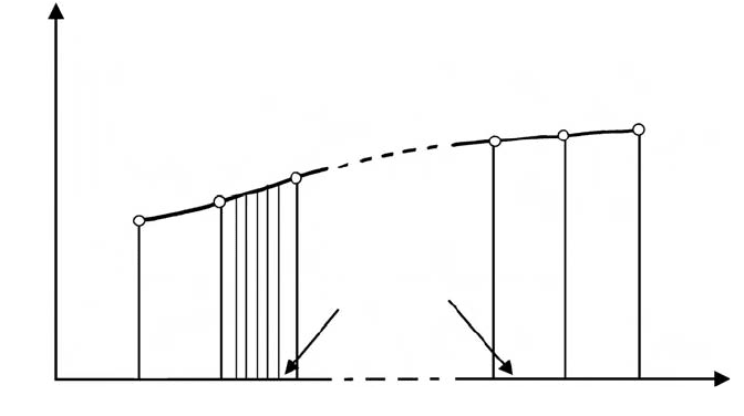
nication point (Fig. 1-2a). Within each integration step, numerical integration

8 Introduction to Dynamic-system Simulation

x (t)

COMINT

t0 t0+COMINT t0+2 COMINT t0+TMAX

FIGURE 1-2

. Time history of a simulation variable, showing sampling times t = t0, t0 +

COMINT, t0 + 2 COMINT, …, t0 + TMAX and some integration steps. In the figure, all integration

steps end on a sampling point. This is always true for variable-step integration rules, but fixed

integration steps

DT may overshoot the sampling points by a small fraction of DT, as shown in

Figure 1-2b.

approximates continuous updating of the “continuous” model variables t, xi,

and

yj. Each integration step usually requires more than one derivative call

executing the model equations (1-1) (Section 1-7; [10–18]).

In DYNAMIC program segments without differential equations,

defaults to t0 = 1 unless the experiment-protocol script specifies a different

value. All operations in such a DYNAMIC segment are sampled-data assign-

ments and execute at successive communication times [Eq. (1-2)], except for

assignments preceded by a

SAMPLE m statement, where m is an integer >1.

Such assignments execute only at

t = t0 and then at every m

communication

point. This permits multirate sampling. DESIRE admits only one

SAMPLE

m statement per DYNAMIC program segment.

Differential-equation-solving DYNAMIC segments can also include sam-

pled-data assignments that execute only at the periodic sampling points (1-2).

Such assignments model sampled-data controllers and noise generators and

must be collected in sections following an

OUT and/or SAMPLE m statement

at the end of the DYNAMIC program segment (Section 2-3).

DYNAMIC-segment input/output (e.g., to displays and listings) occurs at

the

NN communication points (1-2), unless the system variable MM, which

defaults to 1, is set to an integer >1. In this case, input/output occurs at

t = t0,

then at every

sampling point, and finally at t = t0 + TMAX. NN can thus

be set to a larger value than the desired number of input/output points. This

How a Simulation Run Works 9

FIGURE 1-2

. DESIRE output listings for variable-step integration and for fixed-step

integration. Parameters were deliberately chosen to exaggerate the fixed-

DT effect.

Variable-step integration

NN = 6 | TMAX = 10 | initial DT = 0.01

t, x,X,y

0.00000e+00 0.00000e+00 0.00000e+00 0.00000e+00

2.00000e+00 3.89418e-01 3.89418e-01 0.00000e+00

4.00000e+00 7.17356e-01 3.89418e-01 3.89418e-01

6.00000e+00 9.32039e-01 9.32039e-01 3.89418e-01

8.00000e+00 9.99574e-01 9.32039e-01 9.32039e-01

1.00000e+01 9.09298e-01 9.09298e-01 9.32039e-01

Fixed-step integration

NN = 6 | TMAX = 11 | initial DT = 0.01

t, x,X,y

0.00000e+00 0.00000e+00 0.00000e+00 0.00000e+00

2.00000e+00 3.89419e-01 3.89419e-01 0.00000e+00

4.01000e+00 7.18748e-01 3.89419e-01 3.89419e-01

6.01000e+00 9.32762e-01 9.32762e-01 3.89419e-01

8.01000e+00 9.99513e-01 9.32762e-01 9.32762e-01

1.00100e+01 9.08463e-01 9.08463e-01 9.32762e-01

can provide fast sampling for pseudorandom noise (Section 5-4) and/or for

sampling switch and limiter functions (Sections 2-10 and 2-11).

Some defined-variable assignments (1-1b) do not affect state variables but

only scale or modify model output. Such operations are not needed at every

derivative call but only at sampling points. The simulation will run faster if

such assignments are programmed as sampled-data operations following an

OUT statement.

1-7. Numerical Integration

(a) Euler Integration

The simplest procedure that approximates continuous updating of a state

variable x in successive integration steps is the explicit Euler integration rule

(see also Appendix)

xi(t + DT) = xi(t) + fi[t; x1(t), x2(t), ...; y1(t), y2(t),... ]DT

(i = 1, 2, …, n) (1-3)

where

fi is the value of dx/dt calculated by the derivative call executing Eq.

(1-1) at the time

The integration routine loops until

t reaches the next communication point

(1-2), where the solution is sampled for input/output and sampled-data oper-

ations. The simulation run terminates after accessing the last sample at

t = t0 +

TMAX unless the run is stopped either by the user or by a programmed

termination (

term) statement.

(b) Improved Integration Rules

The Euler integration rule [Eq. (1-3)] simply increments each state variable

by an amount proportional to its last computed derivative. This does not

approximate true integration well except for very small integration steps

DT.

Improved updating requires multiple derivative calls per integration step

[10–18]. This can actually reduce the total number of derivative calls (the

main computing load of a simulation) required for a specified accuracy. In

particular:

• Multistep rules extrapolate updated values of the

xi as polynomials based

on values of the

xi and fi at several past times t – DT, t – 2DT, … .

• Runge–Kutta rules precompute two or more approximate derivative values

in the interval

(t, t + DT) by Euler-type steps and use their weighted aver-

age for updating.

10 Introduction to Dynamic-system Simulation

Coefficients in such integration formulas are chosen so that polynomials

of degree

N integrate exactly (N

-order integration formula).

Explicit integration rules such as Eq. (1-3) express future values

xi(t + DT)

in terms of already computed past state-variable values. Implicit rules, such

as the implicit Euler rule,

xi(t + DT) = xi(t) + fi[t + DT; x1(t + DT), x2(t + DT), ...;

y1(t + DT), y2(t + DT), ...] DT (i = 1, 2, ..., n) (1-4)

require a program that solves the predictor equation (1-4) for

xi(t + DT) at

each step. Implicit rules clearly involve more computation, but they may

admit larger

DT values without numerical instability.

Variable-step integration adjusts integration step sizes to maintain accu-

racy estimates obtained by comparing various tentative updated solution val-

ues. This can save many steps. Figures 1-5, 7-7, and 7-8 show examples.

Numerical integration normally assumes integrands

fi that are continuous and

differentiable within each integration step. Step-function inputs are accept-

able only at

t = t0 and thereafter at the end of integration steps. Sections 2-10

to 2-12 discuss this problem in connection with models involving sampled-

data operations and switching functions.

1-8. Sampling Times and Integration Steps

The experiment protocol script selects the simulation runtime

TMAX and the

number of samples

NN needed for display, listings, and/or sampled-data

models. DESIRE returns an error message if an integration-step value

larger than COMINT = TMAX/(NN – 1) is selected, for the program must never

sample data within integration steps. Sampled-data output to displays or sam-

pled-data assignments is not well-defined at such times. Sampled-data input

within integration steps might make the numerical-integration routine invalid

(see also Sections 2-9 to 2-11).

DESIRE’s variable-step integration routines automatically force the last

integration step in each communication interval to end precisely on one of the

user-selected communication points (1-2). An error message warns if the initial

DT value exceeds COMINT. Fixed-step integration routines, however, may

have to add a fraction of

DT to each sampling time (1-2) to make sure that sam-

pling always occurs at the end of an integration step, as shown in Eq. (1-2b).

This does not cause errors in displays or listings, for each

x(t) value is still asso-

ciated with its correct

t value. But if output listings at specified periodic sam-

pling times (1-2) are needed, one must either use variable-step integration or set

DT to a very small integral fraction of COMINT.

How a Simulation Run Works 11