Masujima M. Applied Mathematical Methods in Theoretical Physics
Подождите немного. Документ загружается.


388 10 Calculus of Variations: Applications
iγ
k
∂
k
+ iγ
4
∂
∂τ
− µ
−m + gγ
1
i
δ
δJ(τ ,
x)
β,α
1
i
δ
δη
α
(τ , x)
Z
GC
(β;[J, η, η])
=−η
β
(τ ,
x )Z
GC
(β;[J, η, η]), (10.5.22)
iγ
k
∂
k
+ iγ
4
∂
∂τ
+ µ
+m − gγ
1
i
δ
δJ(τ ,
x)
T
β,α
i
δ
δη
β
(τ ,
x )
Z
GC
(β;[J, η, η])
=
η
α
(τ ,
x )Z
GC
(β;[J, η, η]), (10.5.23)
∂
2
∂x
2
ν
− κ
2
1
i
δ
δJ(τ ,
x )
− gγ
βα
δ
2
δη
α
(τ ,
x)δη
β
(τ ,
x)
Z
GC
(β;[J, η, η])
= J(τ ,
x )Z
GC
(β;[J, η, η]). (10.5.24)
We can solve the functional differential equations, (10.5.22), (10.5.23), and (10.5.24),
by the method discussed in Section 10.3. As in Section 10.3, we define the functional
Fourier transform
˜
Z
GC
(β;[φ, ψ
E
, ψ
E
]) of Z
GC
(β;[J, η, η]) by
Z
GC
(β;[J, η, η]) ≡
D [ψ
E
]D [ψ
E
]D [φ]
˜
Z
GC
(β;[φ, ψ
E
, ψ
E
])
× exp
i
β
0
dτ
d
3
x {J(τ ,
x )φ(τ,
x)
+
η
α
(τ ,
x)ψ
E α
(τ ,
x ) + ψ
E β
(τ ,
x)η
β
(τ ,
x )}
.
We obtain the equations of motion satisfied by the functional Fourier transform
˜
Z
GC
(β;[φ, ψ
E
, ψ
E
]) from Eqs. (10.5.22), (10.5.23), and (10.5.24), after the functional
integral by parts on the right-hand sides involving
η
α
, η
β
,andJ as
δ
δψ
E α
(τ ,
x)
ln
˜
Z
GC
(β;[φ, ψ
E
, ψ
E
]) =
δ
δψ
E α
(τ ,
x )
β
0
dτ
d
3
xL
E
((10.5.1)),
δ
δψ
E β
(τ ,
x)
ln
˜
Z
GC
(β;[φ, ψ
E
, ψ
E
]) =
δ
δψ
E β
(τ ,
x )
β
0
dτ
d
3
xL
E
((10.5.1)),
δ
δφ(τ ,
x)
ln
˜
Z
GC
(β;[φ, ψ
E
, ψ
E
]) =
δ
δφ(τ ,
x )
β
0
dτ
d
3
xL
E
((10.5.1)),
which we can immediately integrate to obtain
˜
Z
GC
(β;[φ, ψ
E
, ψ
E
]) = C exp
β
0
dτ
d
3
x L
E
((10.5.1))
. (10.5.25a)
Thus we have the path integral representation of Z
GC
(β;[J, η, η]) as
Z
GC
(β;[J, η, η]) = C
D [ψ
E
]D [ψ
E
]D [φ]exp
β
0
dτ
d
3
x {L
E
((10.5.1))
+iJ(τ ,
x )φ(τ,
x) + i
η
α
(τ ,
x)ψ
E α
(τ ,
x ) + iψ
E β
(τ ,
x)η
β
(τ ,
x )}

10.5 Schwinger–Dyson Equation in Quantum Statistical Mechanics 389
= Z
0
exp
−gγ
βα
β
0
dτ
d
3
xi
δ
δη
β
(τ ,
x)
1
i
δ
δη
α
(τ ,
x)
1
i
δ
δJ(τ ,
x )
× exp
β
0
dτ
d
3
x
β
0
dτ
d
3
x
−
1
2
J(τ ,
x)D
0
(τ −τ
,
x −
x
)J(τ
,
x
)
+
η
α
(τ ,
x )S
0
αβ
(τ − τ
,
x −
x
)η
β
(τ
,
x
)
. (10.5.25b)
The normalization constant Z
0
is so chosen that
Z
0
= Z
GC
(β;J = η = η = 0, g = 0)
=
$
|
p
|
,
k
{1 + exp[−β(ε
p
−µ)]}{1 +exp[−β(ε
p
+µ)]}{1 −exp[−βω
k
]}
−1
,
(10.5.26)
with
ε
p
= (
p
2
+ m
2
)
1
2
, ω
k
= (
k
2
+ κ
2
)
1
2
. (10.5.27)
D
0
(τ − τ
,
x −
x
)andS
0
αβ
(τ − τ
,
x −
x
) are the ‘‘free’’ temperature Green’s func-
tions of the Bose field and the Fermi field, respectively, and are given by
D
0
(τ − τ
,
x −
x
) =
d
3
k
(2π)
3
2ω
k
{(f
k
+ 1) exp[i
k(
x −
x
) − ω
k
(τ − τ
)]
+ f
k
exp[−i
k(
x −
x
) + ω
k
(τ − τ
)]},
S
0
αβ
(τ −τ
,
x −
x
) = (iγ
ν
∂
ν
+ m)
α,β
d
3
k
(2π)
3
2ε
k
×
{(N
+
k
− 1) exp[i
k(
x −
x
) − (ε
k
− µ)(τ − τ
)]
+N
−
k
exp[−i
k(
x −
x
) +(ε
k
+ µ)(τ − τ
)]},
for τ>τ
,
{N
+
k
exp[−i
k(
x −
x
) −(ε
k
− µ)(τ − τ
)]
+(N
−
k
−1) exp[i
k(
x −
x
) + (ε
k
+ µ)(τ − τ
)]},
for τ<τ
,
∂
4
≡
∂
∂τ
− µ, f
k
=
1
exp[βω
k
] − 1
, N
±
k
=
1
exp[β(ε
k
∓ µ)] +1
.
The f
k
is the density of the state of the Bose particles at energy ω
k
,andtheN
±
k
is
the density of the state of the (anti-)Fermi particles at energy ε
k
.
We have two ways of expressing Z
GC
(β;[J, η, η]), Eq. (10.5.25b):
Z
GC
(β;[J, η, η])
= Z
0
exp
−
1
2
β
0
dτ
d
3
x
β
0
dτ
d
3
x
(
J(τ ,
x) −gγ
βα
i
δ
δη
β
(τ ,
x )

390 10 Calculus of Variations: Applications
×
1
i
δ
δη
α
(τ ,
x)
+
× D
0
(τ − τ
,
x −
x
)
(
J(τ
,
x
) − gγ
βα
i
δ
δη
β
(τ
,
x
)
1
i
δ
δη
α
(τ
,
x
)
+
× exp
β
0
dτ
d
3
x
β
0
dτ
d
3
x
η
α
(τ ,
x)S
0
αβ
(τ − τ
,
x −
x
)η
β
(τ
,
x
)
(10.5.28)
= Z
0
(
Det(1 + gS
0
(τ ,
x )γ
1
i
δ
δJ(τ ,
x)
)
+
−1
exp
β
0
dτ
d
3
x
β
0
dτ
d
3
x
× η
α
(τ ,
x )
1 +gS
0
(τ ,
x )γ
1
i
δ
δJ(τ ,
x )
−1
αε
S
0
εβ
(τ − τ
,
x −
x
)η
β
(τ
,
x
)
× exp
−
1
2
β
0
dτ
d
3
x
β
0
dτ
d
3
x
J(τ ,
x )D
0
(τ − τ
,
x −
x
)J(τ
,
x
)
.
(10.5.29)
The thermal expectation value of the τ-ordered function
f
τ -ordered
(
ˆ
ψ,
&
ψ,
ˆ
φ)
in the grand canonical ensemble is given by
f
τ -ordered
(
ˆ
ψ,
&
ψ,
ˆ
φ)≡
Tr{ˆρ
GC
(β)f
τ -ordered
(
ˆ
ψ,
&
ψ,
ˆ
φ)}
Tr ˆρ
GC
(β)
≡
1
Z
GC
(β;[J, η, η])
× f
1
i
δ
δη
, i
δ
δη
,
1
i
δ
δJ
)Z
GC
(β;[J, η, η]
J=η=η=0
.
(10.5.30)
According to this formula, the one body ‘‘full’’ temperature Green’s functions of
the Bose field and the Fermi field, D(τ − τ
,
x −
x
)andS
αβ
(τ − τ
,
x −
x
), are
given, respectively, by
D(τ − τ
,
x −
x
) =
Tr{ˆρ
GC
(β)T
τ
(
ˆ
φ(τ ,
x)
ˆ
φ(τ
,
x
))}
Tr ˆρ
GC
(β)
=−
1
Z
GC
(β;[J, η, η])
1
i
δ
δJ(τ ,
x)
1
i
×
δ
δJ(τ
,
x
)
Z
GC
(β;[J, η, η])
J=η=η=0
, (10.5.31)

10.5 Schwinger–Dyson Equation in Quantum Statistical Mechanics 391
S
αβ
(τ − τ
,
x −
x
) =
Tr{ˆρ
GC
(β)
ˆ
ψ
α
(τ ,
x )
&
ψ
β
(τ
,
x
)}
Tr ˆρ
GC
(β)
=−
1
Z
GC
(β;[J, η, η])
1
i
×
δ
δη
α
(τ ,
x )
i
δ
δη
β
(τ
,
x
)
Z
GC
(β;[J, η, η])
J=η=η=0
.
(10.5.32)
From the cyclicity of Tr and the (anti-)commutativity of
ˆ
φ(τ ,
x)(
ˆ
ψ
α
(τ ,
x)) under the
T
τ
-ordering symbol, we have
D(τ − τ
< 0,
x −
x
) =+D(τ − τ
+ β,
x −
x
), (10.5.33)
and
S
αβ
(τ − τ
< 0,
x −
x
) =−S
αβ
(τ − τ
+ β,
x −
x
), (10.5.34)
where
0 ≤ τ , τ
≤ β,
i.e., the Boson (Fermion) ‘‘full’’ temperature Green’s function is (anti-)periodic
with the period β. From this, we have the Fourier decompositions as
ˆ
φ(τ ,
x ) =
1
β
n
d
3
k
(2π)
3
2ω
k
/
exp[i(
k
x − ω
n
τ )]a(ω
n
,
k)
+ exp[−i(
k
x − ω
n
τ )]a
†
(ω
n
,
k)
0
, (10.5.35)
ω
n
=
2nπ
β
, n = integer,
ˆ
ψ
α
(τ ,
x ) =
1
β
n
d
3
k
(2π)
3
2ε
k
/
exp[i(
k
x − ω
n
τ )]u
nα
(
k)b(ω
n
,
k)
+exp[−i(
k
x − ω
n
τ )]v
nα
(
k)d
†
(ω
n
,
k)
0
, (10.5.36)
ω
n
=
(2n + 1)π
β
, n = integer,
where
[a(ω
n
,
k), a
†
(ω
n
,
k
)] = 2ω
k
(2π)
3
δ
3
(
k −
k
)δ
n,n
, (10.5.37)
[a(ω
n
,
k), a(ω
n
,
k
)] = [a
†
(ω
n
,
k), a
†
(ω
n
,
k
)] = 0, (10.5.38)
/
b(ω
n
,
k), b
†
(ω
n
,
k
)
0
=
/
d(ω
n
,
k), d
†
(ω
n
,
k
)
0
= 2ε
k
(2π)
3
δ
3
(
k −
k
)δ
n,n
,
(10.5.39)
the rest of anticommutators = 0. (10.5.40)

392 10 Calculus of Variations: Applications
We shall now address ourselves to the problem of finding the equation of motion
of the one-body Boson and Fermion Green’s functions. We define the 1-body Boson
and Fermion ‘‘full’’ temperature Green’s functions, D
J
(x, y)andS
J
α,β
(x, y), by for
Boson field Green’s function:
D
J
(x, y) ≡−T
τ
(
ˆ
φ(x)
ˆ
φ(y))
J
η=η=0
(10.5.41)
≡−
δ
2
δJ(x )δJ(y)
ln Z
GC
(β;[J, η, η])
η=η=0
≡−
δ
δJ(x )
ˆ
φ(y)
J
η=η=0
,
and for Fermion field Green’s function:
S
J
α,β
(x, y) ≡+T
τ
(
ˆ
ψ
α
(x)
&
ψ
β
(y))
J
η=η=0
(10.5.42)
≡−
1
Z
GC
(β;[J, η, η])
δ
δη
α
(x)
δ
δη
β
(y)
Z
GC
(β;[J, η, η])
η=η=0
.
From Eqs. (10.5.22), (10.5.23), and (10.5.24), we obtain a summary of the
Schwinger–Dyson equation satisfied by D
J
(x, y)andS
J
α,β
(x, y):
Summary of Schwinger–Dyson equation in configuration space
(iγ
ν
∂
ν
− m + gγ
ˆ
φ(x)
J
)
αε
S
J
εβ
(x, y) −
d
4
z
∗
αε
(x, z)S
J
εβ
(z, y)
= δ
αβ
δ
4
(x − y),
∂
2
∂x
2
ν
−κ
2
ˆ
φ(x)
J
=
1
2
gγ
βα
/
S
J
αβ
(τ ,
x ;τ − ε,
x ) + S
J
αβ
(τ ,
x ;τ + ε,
x )
0
ε→0
+
,
∂
2
∂x
2
ν
−κ
2
D
J
(x, y) −
d
4
z
∗
(x, z)D
J
(z, y) = δ
4
(x − y),
∗
αβ
(x, y) = g
2
d
4
ud
4
vγ
αδ
S
J
δν
(x, u)
νβ
(u, y;v)D
J
(v, x),
∗
(x, y) = g
2
d
4
ud
4
vγ
αβ
S
J
βδ
(x, u)
δν
(u, v;y)S
J
να
(v, x),
αβ
(x, y;z) = γ
αβ
(z)δ
4
(x − y)δ
4
(x − z) +
1
g
δ
∗
αβ
(x, y)
δ
ˆ
φ(z)
J
.
This system of nonlinear coupled integro-differential equations is exact and
closed. Starting from the 0th-order term of
αβ
(x, y;z), we can develop
Feynman–Dyson-type graphical perturbation theory for quantum statistical
10.5 Schwinger–Dyson Equation in Quantum Statistical Mechanics 393
g
2
g
ad
(x)
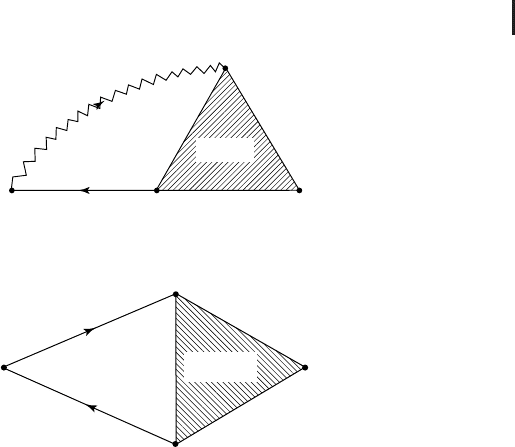
∑ (x, y) =
x, d
u, n
y, b
v
D
J
(v,x)
S
J
d n
(x,u)
Γ (u,y;v)
ab
∗
Fig. 10.9 Graphical representation of the proper self-energy part,
∗
αβ
(x, y).
∗
Γ (u,v;y)
S
J
bd
(x,u)
S
J
na
(v,x)
x, b
Π(x,y) =
g
2
g
ab
(x)
u, d
y
v, n
Fig. 10.10 Graphical representation of the proper self-energy part,
∗
(x, y).
mechanics in the configuration space by iteration. We here employed the following
abbreviation:
x ≡ (τ
x
,
x ),
d
4
x ≡
β
0
dτ
x
d
3
x .
We note that S
J
αβ
(x, y)andD
J
(x, y) are determined by Eqs. (10.5.3a)–(10.5.3f) only
for
τ
x
− τ
y
∈ [−β, β],
and we assume that they are defined by the periodic boundary condition with the
period 2β for other
τ
x
− τ
y
/∈ [−β, β].
Next we set
J ≡ 0,
and hence we have
ˆ
φ(x)
J≡0
≡ 0,
restoring the translational invariance of the system. We Fourier transform S
αβ
(x)
and D(x),

394 10 Calculus of Variations: Applications
S
αβ
(x) =
1
β
p
4
d
3
p
(2π)
3
S
αβ
(p
4
,
p)exp[i(
p
x − p
4
τ
x
)], (10.5.43a)
D(x) =
1
β
p
4
d
3
p
(2π)
3
D(p
4
,
p)exp[i(
p
x − p
4
τ
x
)], (10.5.43b)
α,β
(x, y;z) =
α,β
(x − y, x − z) =
1
β
2
p
4
,k
4
d
3
pd
3
k
(2π)
6
α,β
(p, k)
× exp[i{
p(
x −
y) −p
4
(τ
x
− τ
y
)}−i{
k(
x −
z) −k
4
(τ
x
−τ
z
)}],
(10.5.43c)
p
4
=
(
(2n + 1)π β, Fermion, n = integer,
2nπβ, Boson, n = integer.
(10.5.43d)
We have the Schwinger–Dyson equation in the momentum space:
Summary of Schwinger–Dyson equation in the momentum space
1
−γ
p + γ
4
(p
4
− iµ) −(m +
∗
(p))
2
αε
S
εβ
(p) = δ
αβ
n
δ
p
4
−
(2n + 1)π
β
,
/
− k
2
ν
− (κ
2
+
∗
(k))
0
D(k) =
n
δ
k
4
−
2nπ
β
,
∗
α,β
(p) = g
2
1
β
k
4
d
3
k
(2π)
3
γ
αδ
S
δε
(p + k)
εβ
(p + k, k)D(k),
∗
(k) = g
2
1
β
p
4
d
3
p
(2π)
3
γ
µν
S
νλ
(p + k)
λρ
(p + k, k)S
ρµ
(p),
αβ
(p, k) =
n,,m
γ
αβ
δ
p
4
−
(2n + 1)π
β
δ
k
4
−
(2m + 1)π
β
+
αβ
(p, k),
where
αβ
(p, k) represents the sum of the vertex diagram except for the first term.
This system of nonlinear coupled integral equations is exact and closed. Starting
from the 0th-order term of
αβ
(p, k), we can develop a Feynman–Dyson-type
graphical perturbation theory for quantum statistical mechanics in the momentum
space by iteration.
From the Schwinger–Dyson equation, we can derive the Bethe–Goldstone
diagram rule of the many-body problems at finite temperature in quantum statistical
mechanics, nuclear physics, and condensed matter physics. For details of this
diagram rule, we refer the reader to A.L. Fetter and J.D. Walecka.

10.6 Feynman’s Variational Principle 395
10.6
Feynman’s Variational Principle
In this section, we shall briefly consider Feynman’svariational principle in quantum
statistical mechanics.
We consider the canonical ensemble with the Hamiltonian
ˆ
H({
q
j
,
p
j
}
N
j=1
)at
finite temperature. The density matrix ˆρ
C
(β)ofthissystemsatisfiestheBloch
equation,
−
∂
∂τ
ˆρ
C
(τ ) =
ˆ
H ({
q
j
,
p
j
}
N
j=1
)ˆρ
C
(τ ), 0 ≤ τ ≤ β, (10.6.1)
with its formal solution given by
ˆρ
C
(τ ) = exp[−τ
ˆ
H({
q
j
,
p
j
}
N
j=1
]ˆρ
C
(0). (10.6.2)
We compare the Bloch equation and the density matrix, Eqs. (10.6.1) and (10.6.2),
with the Schr
¨
odinger equation for the state vector
|
ψ, t > ,
i
d
dt
|
ψ, t > =
ˆ
H({
q
j
,
p
j
}
N
j=1
)
|
ψ, t > , (10.6.3)
and its formal solution given by
|
ψ, t > = exp[−it
ˆ
H({
q
j
,
p
j
}
N
j=1
)]
|
ψ,0>. (10.6.4)
We find that by the analytic continuation,
t =−iτ ,0≤ τ ≤ β ≡ k
B
T, (10.6.5)
k
B
= Boltzmann constant, T = absolute temperature,
the (real time) Schr
¨
odinger equation and its formal solution, Eqs. (10.6.3) and
(10.6.4), are analytically continued into the Bloch equation and the density matrix,
Eqs. (10.6.1) and (10.6.2), respectively. By the analytic continuation, Eq. (10.6.5),
we divide the interval [0, β] into the n equal subinterval, and use the resolution
of the identity in both the q-representation and the p-representation. In this way,
we obtain the following list of correspondence. Here, we assume the Hamiltonian
ˆ
H({
q
j
,
p
j
}
N
j=1
) of the following form:
ˆ
H ({
q
j
,
p
j
}
N
j=1
) =
N
j=1
1
2m
p
2
j
+
j>k
V(
q
j
,
q
k
). (10.6.6)

396 10 Calculus of Variations: Applications
List of Correspondence
Quantum mechanics Quantum statistical mechanics
Schr
¨
odinger equation
i
∂
∂t
|
ψ, t >
= H ({
q
j
,
p
j
}
N
j=1
)
|
ψ, t >.
Bloch equation
−
∂
∂τ
ˆρ
C
(τ )
= H ({
q
j
,
p
j
}
N
j=1
)ˆρ
C
(τ ).
Schr
¨
odinger state vector
|
ψ, t >
= exp[−itH({
q
j
,
p
j
}
N
j=1
)]
|
ψ,0>.
Density matrix
ˆρ
C
(τ )
= exp[−τ H({
q
j
,
p
j
}
N
j=1
)]ˆρ
C
(0).
Minkowskian Lagrangian
L
M
({q
j
(t),
˙
q
j
(t)}
N
j=1
)
=
#
N
j=1
1
2
m
˙
q
2
j
(t)
−
#
N
j>k
V(
q
j
,
q
k
).
Euclidean Lagrangian
L
E
({q
j
(τ ),
˙
q
j
(τ )}
N
j=1
)
=−
#
N
j=1
1
2
m
˙
q
2
j
(τ )
−
#
N
j>k
V(
q
j
,
q
k
).
i × Minkowskian action
functional
iI
M
[{
q
j
}
N
j=1
;
q
f
,
q
i
]
= i
3
t
f
t
i
dtL
M
({q
j
(t),
˙
q
j
(t)}
N
j=1
).
Euclidean action
functional
I
E
[{
q
j
}
N
j=1
;
q
f
,
q
i
]
=
3
β
0
dτ L
E
({q
j
(τ ),
˙
q
j
(τ )}
N
j=1
).
Transformation function
q
f
, t
f
q
i
, t
i
=
3
q(t
f
)=
q
f
q(t
i
)=
q
i
D [
q]×
×exp[iI
M
[{
q
j
}
N
j=1
;
q
f
,
q
i
]].
Transformation function
Z
f ,i
=
3
q(β)=
q
f
q(0)=
q
i
D [
q]×
×exp[I
E
[{
q
j
}
N
j=1
;
q
f
,
q
i
]].
Vacuum-to-vacuum
transition amplitude
0, out
|
0, in
=
3
D [
q]exp[iI
M
[{
q
j
}
N
j=1
]].
Partition function∗
Z
C
(β) = Tr ˆρ
C
(β)
= ‘‘
3
d
q
f
d
q
i
δ(
q
f
−
q
i
)Z
f ,i
’’.
Vacuum expectation value
O(
ˆ
q)
=
3
D [
q]O(
q)exp[iI
M
[{
q
j
}
N
j=1
]]
3
D [
q]exp{iI
M
[{
q
j
}
N
j=1
]}
.
Thermal expectation value*
O(
ˆ
q)
=
Tr ˆρ
C
(β)O(
ˆ
q)
Tr ˆρ
C
(β)
.
In the list above, entries with ‘‘*’’ are given, respectively, by
Partition function:
Z
C
(β) = Tr ˆρ
C
(β) = ‘‘
d
3
q
f
d
3
q
i
δ
3
(
q
f
−
q
i
)Z
f ,i
’’
=
1
N!
P
δ
P
d
3
q
f
d
3
q
i
δ
3
(
q
f
−
q
Pi
)Z
f ,Pi
=
1
N!
P
δ
P
d
3
q
f
d
3
q
Pi
δ
3
(
q
f
−
q
Pi
)
×
q(β)=
q
f
q(0)=
q
Pi
D [
q]exp[I
E
[{
q
j
}
N
j=1
;
q
f
,
q
Pi
]], (10.6.7)

10.6 Feynman’s Variational Principle 397
Thermal expectation value:
ˆ
O(
q)=
Tr ˆρ
C
(β)
ˆ
O(
ˆ
q)
Tr ˆρ
C
(β)
=
‘‘
3
d
3
q
f
d
3
q
i
δ
3
(
q
f
−
q
i
)Z
f ,i
i
|
O(
q)
f ’’
3
d
3
q
f
d
3
q
i
δ
3
(
q
f
−
q
i
)Z
f ,i
=
1
Z
C
(β)
1
N!
P
δ
P
d
3
q
f
d
3
q
Pi
δ
3
(
q
f
−
q
Pi
)Z
f ,Pi
q
Pi
ˆ
O(
q)
q
f
. (10.6.8)
Here,
q
i
and
q
f
represent the initial position {
q
j
(0)}
N
j=1
and the final position
{
q
j
(β)}
N
j=1
of N identical particles, P represents the permutation of {1, ..., N}, Pi
represents the permutation of the initial position {
q(0)}
N
j=1
and δ
P
represents the
signature of the permutation P, respectively.
In this manner, we obtain the path integral representation of the partition func-
tion, Z
C
(β), and the thermal expectation value,
ˆ
O(
q).FunctionalI
E
[{
q
j
}
N
j=1
;
q
f
,
q
i
]
of Eq. (10.6.7) can be obtained from I
M
[{
q
j
}
N
j=1
;
q
f
,
q
i
]byreplacingt with −iτ .Since
ˆρ
C
(β) is a solution of Eq. (10.6.1), the asymptotic form of Z
C
(β)foralargeτ interval
from τ
i
to τ
f
is
Z
C
(β) ∼ exp[−E
0
(τ
f
− τ
i
)]asτ
f
− τ
i
−→ ∞ .
Therefore, we must estimate Z
C
(β) for large τ
f
− τ
i
.
We choose any real I
1
which approximates I
E
[{
q
j
}
N
j=1
;
q
f
,
q
i
]andwriteZ
C
(β)as
D [
q(ζ )] exp[I
E
[{
q
j
}
N
j=1
;
q
f
,
q
i
]]
=
D [
q(ζ )] exp[(I
E
[{
q
j
}
N
j=1
;
q
f
,
q
i
] − I
1
)]exp[I
1
]. (10.6.9)
The expression (10.6.9) can be regarded as the average of exp[(I
E
− I
1
)]with
respect to the positive weight exp[I
1
]. This observation motivates the variational
principle based on Jensen’s inequality. Since the exponential function is convex,
for any real quantities f , the average of exp[f ] exceeds the exponential of the
average f ,
exp[f ]≥exp[f ]. (10.6.10)
Hence, if in Eq. (10.6.9) we replace I
E
[{
q
j
}
N
j=1
;
q
f
,
q
i
] − I
1
by its average
I
E
[{
q
j
}
N
j=1
;
q
f
,
q
i
] − I
1
=
3
D [
q(ζ )] (I
E
[{
q
j
}
N
j=1
;
q
f
,
q
i
] − I
1
)exp[I
1
]
3
D [
q(ζ )] exp[I
1
]
,
(10.6.11)