Masujima M. Applied Mathematical Methods in Theoretical Physics
Подождите немного. Документ загружается.

24 1 Function Spaces, Linear Operators, and Green’s Functions
a
y
− e
y
y
+ e
b
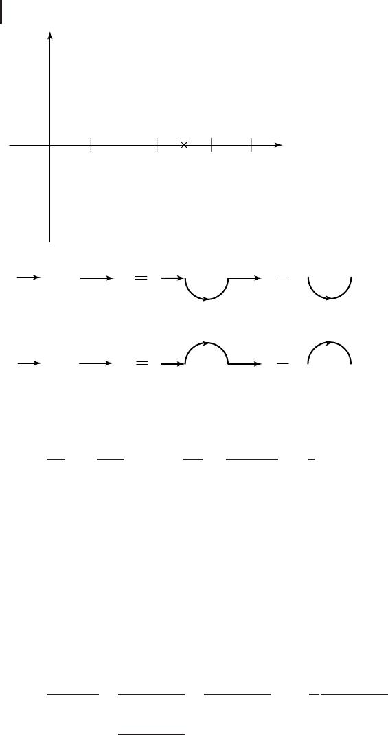
Fig. 1.5 The principal value integral contour.
a
y
− e
y
+ e
b
Fig. 1.6 Two contours for the principal value integral (1.8.13).
Mathematically expressed, the principal value integral is given by either of the
following formulas, known as the Plemelj formula:
1
2πi
P
b
a
f (x)
x − y
dx = lim
ε→0
+
1
2πi
b
a
f (x)
x − y ∓ iε
dx ∓
1
2
f (y), (1.8.14)
This is customarily written as
lim
ε→0
+
1
x − y ∓ iε
= P(1(x − y)) ± iπδ(x − y), (1.8.15a)
or equivalently written as
P(1(x − y )) = lim
ε→0
+
1
x − y ∓ iε
∓ iπδ(x − y ). (1.8.15b)
Then we interchange the order of the limit ε → 0
+
and the integration over x.The
principal value integrand seems to diverge at x = y, but it is actually finite at x = y
as long as f (x) is not singular at x = y. This comes about as follows:
1
x − y ∓ iε
=
(x − y) ± iε
(x − y)
2
+ ε
2
=
(x − y)
(x − y)
2
+ ε
2
±iπ ·
1
π
ε
(x − y)
2
+ ε
2
=
(x − y)
(x − y)
2
+ ε
2
± iπδ
ε
(x − y), (1.8.16)

1.9 Review of Fourier Transform 25
where δ
ε
(x − y)isdefinedby
δ
ε
(x − y) ≡
1
π
ε
(x − y)
2
+ ε
2
, (1.8.17)
with the following properties:
δ
ε
(x = y) → 0
+
as ε → 0
+
; δ
ε
(x = y) =
1
π
1
ε
→+∞ as ε → 0
+
,
+∞
−∞
δ
ε
(x − y)dx = 1.
The first term on the right-hand side of Eq. (1.8.16) vanishes at x = y before we
take the limit ε → 0
+
, while the second term δ
ε
(x − y) approaches the Dirac delta
function, δ(x − y), as ε → 0
+
. This is the content of Eq. (1.8.15a).
1.9
Review of Fourier Transform
The Fourier transform of a function f (x ), where −∞ < x < ∞,isdefinedas
˜
f (k) =
∞
−∞
dx exp[−ikx ] f (x). (1.9.1)
There are two distinct theories of the Fourier transforms.
(I) Fourier transform of square-integrable functions.
It is assumed that
∞
−∞
dx
f (x)
2
< ∞. (1.9.2)
The inverse Fourier transform is given by
f (x) =
∞
−∞
dk
2π
exp[ikx]
˜
f (k). (1.9.3)
We note that in this case
˜
f (k)isdefinedforrealk. Accordingly, the inver-
sion path in Eq. (1.9.3) coincides with the entire real axis. It should be borne
in mind that Eq. (1.9.1) is meaningful in the sense of the convergence in
the mean, namely, Eq. (1.9.1) means that there exists
˜
f (k)forallrealk such
that
lim
R→∞
∞
−∞
dk
˜
f (k) −
R
−R
dx exp[−ikx] f (x)
2
= 0. (1.9.4)

26 1 Function Spaces, Linear Operators, and Green’s Functions
Symbolically we write
˜
f (k) = lim
R→∞
R
−R
dx exp[−ikx ] f (x). (1.9.5)
Similarly in Eq. (1.9.3), we mean that, given
˜
f (k), there exists an f (x )suchthat
lim
R→∞
∞
−∞
dx
f ( f ) −
R
−R
dk
2π
exp[ikx ]
˜
f (k)
2
= 0. (1.9.6)
We can then prove that
∞
−∞
dk
˜
f (k)
2
= 2π
∞
−∞
dx
f (x)
2
. (1.9.7)
This is Parseval’s identity for the square-integrable functions. We see that the pair
( f (x),
˜
f (k)) defined this way consists of two functions with very similar properties.
We shall find that this situation may change drastically if condition (1.9.2) is
relaxed.
(II) Fourier transform of integrable functions.
We relax the condition on the function f (x)as
∞
−∞
dx
f (x)
< ∞. (1.9.8)
Then we can still define
˜
f (k)forrealk. Indeed, from Eq. (1.9.1), we obtain
˜
f (k: real)
=
∞
−∞
dx exp[−ikx] f (x)
≤
∞
−∞
dx
exp[−ikx] f (x)
=
∞
−∞
dx
f (x)
< ∞. (1.9.9)
We can further show that the function defined by
˜
f
+
(k) =
0
−∞
dx exp[−ikx ] f (x) (1.9.10)
is analytic in the upper half-plane of the complex k plane, and
˜
f
+
(k) → 0as
k
→∞ with Im k > 0. (1.9.11)
Similarly, we can show that the function defined by
˜
f
−
(k) =
∞
0
dx exp[−ikx ] f (x) (1.9.12)

1.9 Review of Fourier Transform 27
is analytic in the lower half-plane of the complex k plane, and
˜
f
−
(k) → 0as
k
→∞ with Im k < 0. (1.9.13)
Clearly we have
˜
f (k) =
˜
f
+
(k) +
˜
f
−
(k), k:real. (1.9.14)
We can show that
˜
f (k) → 0ask →±∞, k:real. (1.9.15)
This is a property in common with the Fourier transform of the square-integrable
functions.
Example 1.2. Find the Fourier transform of the following function:
f (x) =
sin(ax)
x
, a > 0, −∞ < x < ∞. (1.9.16)
Solution. The Fourier transform
˜
f (k)isgivenby
˜
f (k) =
∞
−∞
dx exp[ikx]
sin(ax)
x
=
∞
−∞
dx exp[ikx]
exp[iax] − exp[−iax]
2ix
=
∞
−∞
dx
exp[i(k + a)x] − exp[i(k − a)x]
2ix
= I(k + a) − I(k − a),
where we define the integral I(b)by
I(b ) ≡
∞
−∞
dx
exp[ibx]
2ix
=
dx
exp[ibx]
2ix
.
The contour extends from x =−∞to x =∞with the infinitesimal indent below
the real x-axis at the pole x = 0. Noting that x = Re x + i Im x for the complex x,
we have
I(b ) =
2πi · Res
exp[ibx]
2ix
x=0
= π, b > 0,
0, b < 0.
Thus we have
˜
f (k) = I(k + a) − I(k − a) =
∞
−∞
dx exp[ikx]
sin(ax)
x
=
π for
k
< a,
0for
k
> a,
(1.9.17)

28 1 Function Spaces, Linear Operators, and Green’s Functions
while at k =±a,wehave
˜
f (k =±a) =
π
2
,
which is equal to
1
2
[
˜
f (k =±a
+
) +
˜
f (k =±a
−
)].
Example 1.3. Find the Fourier transform of the following function:
f (x) =
sin(ax)
x (x
2
+ b
2
)
, a, b > 0, −∞ < x < ∞. (1.9.18)
Solution. The Fourier transform
˜
f (k)isgivenby
˜
f (k) =
dz
exp[i(k + a)z]
2iz(z
2
+ b
2
)
−
dz
exp[i(k − a)z]
2iz(z
2
+ b
2
)
= I(k + a) − I(k − a),
(1.9.19a)
where we define the integral I(c)by
I(c) ≡
∞
−∞
dz
exp[icz]
2iz(z
2
+b
2
)
=
dz
exp[icz]
2iz(z
2
+ b
2
)
, (1.9.19b)
where the contour is the same as in Example 1.2. The integrand has the simple
poles at
z = 0andz =±ib.
Noting z = Re z + i Im z,wehave
I(c) =
2πi · Res
exp[icz]
2iz(z
2
+b
2
)
z=0
+ 2π i · Res
exp[icz]
2iz(z
2
+b
2
)
z=ib
, c > 0,
−2πi · Res
exp[icz]
2iz(z
2
+b
2
)
z=−ib
, c < 0,
or
I(c) =
(π2b
2
)(2 − exp[−bc]), c > 0,
(π2b
2
)exp[bc], c < 0.
Thus we have
˜
f (k) = I(k + a) −I(k − a) =
(πb
2
)sinh(ab)exp[bk], k < −a,
(πb
2
){1 − exp[−ab]cosh(bk)},
k
< a,
(πb
2
)sinh(ab)exp[−bk], k > a.
(1.9.20)

1.9 Review of Fourier Transform 29
We note that
˜
f (k)isstep-discontinuous at k =±a inExample1.2.Wealsonotethat
˜
f (k)and
˜
f
(k)arecontinuous for real k,while
˜
f
(k)isstep-discontinuous at k =±a in
Example 1.3.
We note that the rate with which
f (x) → 0as
|
x
|
→+∞
affects the degree of smoothness of
˜
f (k). For the square-integrable functions, we
usually have
f (x) = O
1
x
as
|
x
|
→+∞⇒
˜
f (k) step-discontinuous,
f (x) = O
1
x
2
as
|
x
|
→+∞⇒
˜
f (k) continuous,
˜
f
(k) step-discontinuous,
f (x) = O
1
x
3
as
|
x
|
→+∞⇒
˜
f (k),
˜
f
(k) continuous,
˜
f
(k) step-discontinuous,
and so on.
Having learned in above the abstract notions relating to linear space, inner
product, operator and its adjoint, eigenvalue and eigenfunction, Green’s function,
and the review of Fourier transform and complex analysis, we are now ready to
embark on our study of integral equations. We encourage the reader to make an
effort to connect the concrete example that will follow with the abstract idea of linear
function space and linear operator. This will not be possible in all circumstances.
The abstract idea of function space is also useful in the discussion of the calculus
of variations where a piecewise continuous but nowhere differentiable function
and a discontinuous function show up as the solution of the problem.
We present the applications of the calculus of variations to theoretical physics,
specifically, classical mechanics, canonical transformation theory, the Hamil-
ton–Jacobi equation, classical electrodynamics, quantum mechanics, quantum
field theory and quantum statistical mechanics.
The mathematically oriented reader is referred to the monographs by R. Kress,
and I.M. Gelfand ,andS.V. Fomin for details of the theories of integral equations
and calculus of variations.

31
2
Integral Equations and Green’s Functions
2.1
Introduction to Integral Equations
An integral equation is the equation in which function to be determined appears
in an integral. There exist several types of integral equations:
Fredholm integral equation of the second kind:
φ(x) = F(x) +λ
b
a
K(x, y)φ(y)dy (a ≤ x ≤ b),
Fredholm integral equation of the first kind:
F(x) =
b
a
K(x, y)φ(y)dy (a ≤ x ≤ b),
Volterra integral equation of the second kind:
φ(x) = F(x) +λ
x
0
K(x, y)φ(y)dy with K(x, y) = 0fory > x,
Volterra integral equation of the first kind:
F(x) =
x
0
K(x, y)φ(y)dy with K(x, y) = 0fory > x.
In the above, K(x, y)isthekernel of the integral equation and φ(x) is the unknown
function. If F(x) = 0, the equations are said to be homogeneous,andifF(x) = 0,
they are said to be inhomogeneous.
Now, begin with some simple examples of Fredholm Integral Equations.
Example 2.1. Inhomogeneous Fredholm Integral Equation of the second kind.
φ(x) = x + λ
1
−1
xyφ(y)dy, −1 ≤ x ≤ 1. (2.1.1)
Applied Mathematical Methods in Theoretical Physics, Second Edition. Michio Masujima
Copyright
2009 WILEY-VCH Verlag GmbH & Co. KGaA, Weinheim
ISBN: 978-3-527-40936-5

32 2 Integral Equations and Green’s Functions
Solution. Since
1
−1
yφ(y)dy is some constant, define
A =
1
−1
yφ(y)dy. (2.1.2)
Then Eq. (2.1.1) takes the form
φ(x) = x(1 +λA). (2.1.3)
Substituting Eq. (2.1.3) into the right-hand side of Eq. (2.1.2), we obtain
A =
1
−1
(1 +λA)y
2
dy =
2
3
(1 +λA).
Solving for A,weobtain
1 −
2
3
λ
A =
2
3
.
If λ =
3
2
,nosuchA exists. Otherwise A is uniquely determined to be
A =
2
3
/
1 −
2
3
λ
. (2.1.4)
Thus, if λ =
3
2
, no solution exists. Otherwise, a unique solution exists and is given
by
φ(x) = x/
1 −
2
3
λ
. (2.1.5)
We now consider the homogeneous counter part of the inhomogeneous Fredholm
integral equation of the second kind considered in Example 2.1
Example 2.2. Homogeneous Fredholm Integral Equation of the second kind.
φ(x) = λ
1
−1
xyφ(y)dy, −1 ≤ x ≤ 1. (2.1.6)
Solution. As in Example 2.1, define
A =
1
−1
yφ(y)dy. (2.1.7)
Then
φ(x) = λAx. (2.1.8)

2.1 Introduction to Integral Equations 33
Substituting Eq. (2.1.8) into Eq. (2.1.7), we obtain
A =
1
−1
λAy
2
dy =
2
3
λA. (2.1.9)
The solution exists only when λ =
3
2
. Thus the nontrivial homogeneous solution
exists only for λ =
3
2
, whence φ(x)isgivenbyφ(x) = αx with α arbitrary. If λ =
3
2
,
no nontrivial homogeneous solution exists.
We observe the following correspondence in Examples 2.1 and 2.2:
Inhomogeneous case Homogeneous case
λ = 3/2 Unique solution Trivial solution
λ = 3/2 No solution Infinitely many solutions
(2.1.10)
We further note the analogy of an integral equation to a system of inhomogeneous
linear algebraic equations (matrix equations):
(K − µI)
U =
F (2.1.11)
where K is an n × n matrix, I is the n ×n identity matrix,
U and
F are n-dimensional
vectors, and µ is a number. Equation (2.1.11) has the unique solution,
U = (K − µI)
−1
F, (2.1.12)
provided that (K − µI)
−1
exists, or equivalently that
det(K − µI) = 0. (2.1.13)
The homogeneous equation corresponding to Eq. (2.1.11) is
(K − µI)
U = 0orK
U = µ
U, (2.1.14)
which is the eigenvalue equation for the matrix K. The solutions to the
homogeneous equation (2.1.14) exist for certain values of µ = µ
n
, which are called
the eigenvalues. If µ is equal to an eigenvalue µ
n
,(K − µI)
−1
fails to exist and
Eq. (2.1.11) has generally no finite solution.
Example 2.3. Change the inhomogeneous term x of Example 2.1 to 1.
φ(x) = 1 +λ
1
−1
xyφ(y)dy, −1 ≤ x ≤ 1. (2.1.15)
Solution. As before, define
A =
1
−1
yφ(y)dy. (2.1.16)

34 2 Integral Equations and Green’s Functions
Then
φ(x) = 1 +λAx. (2.1.17)
Substituting Eq. (2.1.17) into Eq. (2.1.16), we obtain A =
1
−1
y(1 +λAy)dy =
2
3
λA.
Thus, for λ =
3
2
, the unique solution exists with A = 0, and φ
(
x
)
= 1, while for
λ =
3
2
, infinitely many solutions exist with A arbitrary and φ
(
x
)
= 1 +
3
2
Ax.
The above three examples illustrate the Fredholm Alternative:
For λ =
3
2
, the homogeneous problem has a solution, given by
φ
H
(x) = αx for any α.
For λ =
3
2
, the inhomogeneous problem has a unique solution, given by
φ(x) =
x /
1 −
2
3
λ
when F
(
x
)
= x ,
1whenF
(
x
)
= 1.
For λ =
3
2
, the inhomogeneous problem has no solution when F(x) = x,while
it has infinitely many solutions when F(x) = 1. In the former case, (φ
H
, F) =
1
−1
αx · xdx = 0, while in the latter case, (φ
H
, F) =
1
−1
αx · 1dx = 0.
It is not surprising that Eq. (2.1.15) has infinitely many solutions when λ = 3/2.
Generally, if φ
0
is a solution of an inhomogeneous equation, and φ
1
is a solution
of the corresponding homogeneous equation, then φ
0
+ aφ
1
is also a solution of
the inhomogeneous equation, where a is any constant. Thus, if λ is equal to an
eigenvalue, an inhomogeneous equation has infinitely many solutions as long
as it has one solution. The nontrivial question is: Under what condition can we
expect the latter to happen? In the present example, the relevant condition is
1
−1
ydy = 0, which means that the inhomogeneous term (which is 1) multiplied
by y and integrated from −1 to 1, is zero. There is a counterpart of this condition
for matrix equations. It is well known that, under certain circumstances, the
inhomogeneous matrix equation (2.1.11) has solutions even if µ is equal to an
eigenvalue. Specifically this happens if the inhomogeneous term
F is a linear
superposition of the vectors each of which forms a column of (K − µI). There is
another way to phrase this. Consider all vectors
V satisfying
(K
T
− µI)
V = 0, (2.1.18)
where K
T
is the transpose of K. The equation above says that
V is an eigenvector of
K
T
with the eigenvalue µ.Italsosaysthat
V is perpendicular to all row vectors of
(K
T
− µI). If
F is a linear superposition of the column vectors of (K − µI)(which
are the row vectors of (K
T
− µI)), then
F is perpendicular to
V. Therefore, the
inhomogeneous equation (2.1.11) has solutions when µ is an eigenvalue, if and
only if
F is perpendicular to all eigenvectors of K
T
with eigenvalue µ. Similarly
an inhomogeneous integral equation has solutions even when λ is equal to an
eigenvalue, as long as the inhomogeneous term is perpendicular to all of the