Masujima M. Applied Mathematical Methods in Theoretical Physics
Подождите немного. Документ загружается.


2.3 Sturm–Liouville System 45
This is a homogeneous Fredholm integral equation of the second kind once G(x, x
)
is known.
Solution for G(x, x
). Recalling Eqs. (2.3.12), (2.3.13), and (2.3.14), we have
G(x, x
) =
Ay
1
(x) + By
2
(x)forx < x
,
Cy
1
(x) + Dy
2
(x)forx > x
.
From the boundary conditions (2.3.14) of G(x, x
), and (2.3.12) and (2.3.13) of y
1
(x)
and y
2
(x), we immediately have
B = 0andC = 0.
Thus we have
G(x, x
) =
Ay
1
(
x
)
for x < x
,
Dy
2
(
x
)
for x > x
.
In order to determine A and D, integrate Eq. (2.3.16) across x
with respect to x,
and make use of the continuity of G(x, x
)atx = x
,whichresultsin
p(x
)
dG
dx
(x
+
, x
) −
dG
dx
(x
−
, x
)
= 1,
G(x
+
, x
) = G(x
−
, x
),
or
Ay
1
(x
) = Dy
2
(x
),
Dy
2
(x
) = Ay
1
(x
)p(x
).
Noting that
W(y
1
(x), y
2
(x)) ≡ y
1
(x)y
2
(x) − y
2
(x)y
1
(x) (2.3.18)
is the Wronskian of the differential equation (2.3.11), we obtain A and D as
A = y
2
(x
)/[p(x
)W(y
1
(x
), y
2
(x
))],
D = y
1
(x
)/[p(x
)W(y
1
(x
), y
2
(x
)].
Now, it can be easily proven that
p(x)W(y
1
(x), y
2
(x)) = constant, (2.3.19)
for the differential equation (2.3.11). Denoting this constant by
p(x)W(y
1
(x), y
2
(x)) = C
,
46 2 Integral Equations and Green’s Functions
we simplify A and D as
A = y
2
(x
)/C
,
D = y
1
(x
)/C
.
Thus Green’s function G(x, x
) for the Sturm–Liouville system is given by
G(x, x
) =
y
1
(
x
)
y
2
x
/C
for x < x
,
y
1
x
y
2
(
x
)
/C
for x > x
,
(2.3.20a)
= y
1
(x
<
)y
2
(x
>
)/C
for
x
<
= ((x + x
)/2) −
x − x
/2,
x
>
= ((x + x
)/2) +
x − x
/2.
(2.3.20b)
The Sturm–Liouville eigenvalue problem is equivalent to the homogeneous
Fredholm integral equation of the second kind,
φ(x) = λ
1
0
G(ξ, x)r(ξ )φ(ξ )dξ. (2.3.21)
We remark that the Sturm–Liouville eigenvalue problem turns out to have a
complete set of eigenfunctions in the space L
2
(0, 1) as long as p(x)andr(x)are
analytic and positive on (0, 1).
The kernel of Eq. (2.3.21) is
K(ξ, x ) = r(ξ)G(ξ , x).
This kernel can be symmetrized by defining
ψ(x) =
r(x)φ(x).
Then the integral equation (2.3.21) becomes
ψ(x) = λ
1
0
r(ξ )G(ξ , x)
r(x)ψ(ξ )dξ. (2.3.22)
Now, the kernel of Eq. (2.3.22),
r(ξ )G(ξ , x)
r(x),
is symmetric since G(ξ, x) is symmetric.
Symmetry of Green’s function, called reciprocity, is true in general for any self-adjoint
operator. The proof of this fact is as follows: consider
L
x
G(x, x
) = δ(x − x
), (2.3.23)

2.4 Green’s Function for Time-Dependent Scattering Problem 47
L
x
G(x, x
) = δ(x − x
). (2.3.24)
Take the inner product of Eq. (2.3.23) with G(x, x
) from the left and Eq. (2.3.24)
with G(x, x
) from the right.
(G(x, x
), L
x
G(x, x
)) = (G(x, x
), δ(x −x
)),
(L
x
G(x, x
), G(x, x
)) = (δ(x − x
), G(x, x
)).
Since L
x
is assumed to be self-adjoint, subtracting the above two equations results
in
G
∗
(x
, x
) = G(x
, x
). (2.3.25)
Then G is Hermitian. If G is real, we have
G(x
, x
) = G(x
, x
),
i.e., G(x
, x
) is symmetric.
2.4
Green’s Function for Time-Dependent Scattering Problem
The time-dependent Schr
¨
odinger equation assumes the following form after setting
= 1and2m = 1:
i
∂
∂t
+
∂
2
∂x
2
ψ(x, t) = V(x, t)ψ(x, t). (2.4.1)
Assume
lim
|
t
|
→∞
V(x, t) = 0,
lim
t→−∞
exp [iω
0
t]ψ(x, t) = exp [ik
0
x ],
(2.4.2)
from which we find
ω
0
= k
2
0
. (2.4.3)
Define Green’s function G(x, t;x
, t
)byrequiring
ψ(x, t) = exp[i(k
0
x − k
2
0
t)]
+
+∞
−∞
dt
+∞
−∞
dx
G(x, t;x
, t
)V(x
, t
)ψ(x
, t
). (2.4.4)
48 2 Integral Equations and Green’s Functions
In order to satisfy partial differential equation (2.4.1), we require
i
∂
∂t
+
∂
2
∂x
2
G(x, t;x
, t
) = δ(t − t
)δ(x − x
). (2.4.5)
We also require that
G(x, t;x
, t
) = 0fort < t
. (2.4.6)
Note that the initial condition at t =−∞is satisfied as well as Causality.Notealso
that the set of equations could be obtained by the methods we were employing in
the previous two examples. To solve the above equations, Eqs. (2.4.5) and (2.4.6),
we Fourier transform in time and space, i.e., we write
˜
G(k, ω;x
, t
) =
+∞
−∞
dx
+∞
−∞
dte
−ikx
e
−iωt
G(x, t;x
, t
),
G(x, t;x
, t
) =
+∞
−∞
dk
2π
+∞
−∞
dω
2π
e
+ikx
e
+iωt
˜
G(k, ω;x
, t
).
(2.4.7)
Taking the Fourier transform of the original equation (2.4.5), we find
G(x, t;x
, t
) =
+∞
−∞
dk
2π
+∞
−∞
dω
2π
−1
ω + k
2
e
ik(x−x
)
e
iω(t−t
)
. (2.4.8)
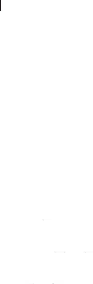
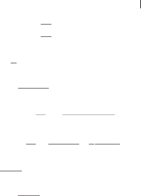
Where do we use the condition that G(x, t;x
, t
) = 0fort < t
?Considertheω
integration in the complex ω plane as in Figure 2.1,
+∞
−∞
dω
1
ω + k
2
e
iω(t−t
)
. (2.4.9)
w
2
w
1
−
k
2
w
Fig. 2.1 The location of the singularity of the integrand
of Eq. (2.4.9) in the complex ω plane.
2.4 Green’s Function for Time-Dependent Scattering Problem 49
We find that there is a singularity right on the path of integration at ω =−k
2
.We
either have to go above or below it. Upon writing ω as ω = ω
1
+ iω
2
,wehavethe
following bound:
e
iω(t−t
)
=
e
iω
1
(t−t
)
e
−ω
2
(t−t
)
= e
−ω
2
(t−t
)
. (2.4.10)
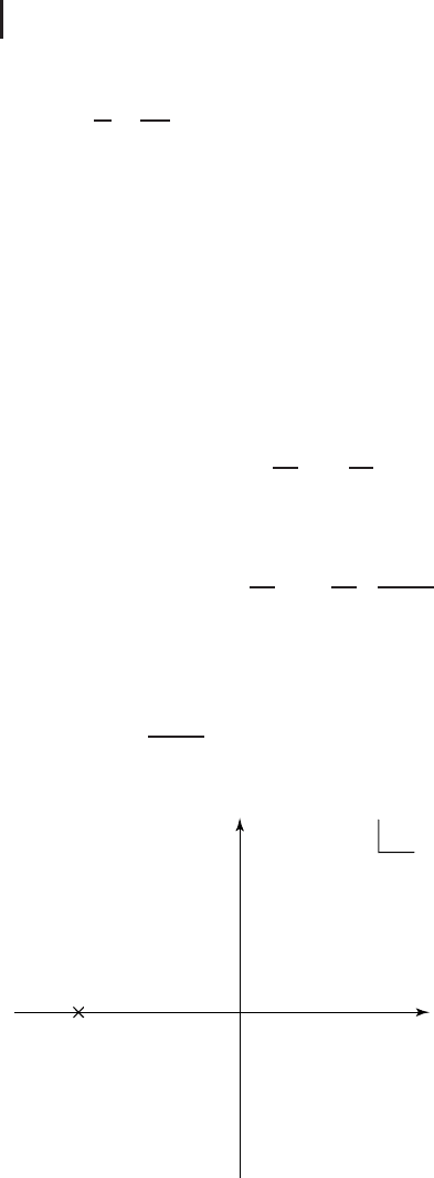
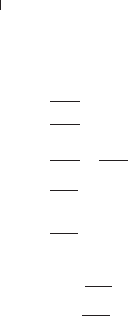
For t < t
, we close the contour in the lower half plane to do the contour integral.
SincewewantG to be zero in this case, we want no singularities inside the contour
in that case. This prompts us to take the contour to be as in Figure 2.2. For t > t
,
when we close the contour in the upper half plane, we get the contribution from
the pole at ω =−k
2
.
The result of calculation is given by
+∞
−∞
dω
1
ω + k
2
e
iω(t−t
)
=
2πi · e
ik(x−x
)−ik
2
(t−t
)
, t > t
,
0, t < t
.
(2.4.11)
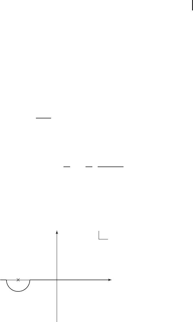
We remark that the idea of the deformation of the contour to satisfy causality is
often expressed by taking the singularity to be at −k
2
+ iε (ε>0) as in Figure 2.3,
whence we replace the denominator ω + k
2
with ω + k
2
− iε,
G(x, t;x
, t
) =
+∞
−∞
dk
2π
+∞
−∞
dω
2π
−1
ω + k
2
− iε
e
ik(x−x
)+iω(t−t
)
. (2.4.12)
This shifts the singularity above the real axis and is equivalent, as ε → 0
+
,toour
previous solution. After the ω integration in the complex ω plane is performed, the
k integral can be done by completing the square in the exponent of Eq. (2.4.12),
but the resulting Gaussian integration is a bit more complicated than the diffusion
equation.
w
2
w
1
w
−
k
2
Fig. 2.2 The contour of the complex ω integration of Eq. (2.4.9).
50 2 Integral Equations and Green’s Functions
−
k
2
+
i
e
w
2
w
w
1
Fig. 2.3 The singularity of the integrand of Eq. (2.4.9) at
ω =−k
2
gets shifted to ω =−k
2
+ iε (ε>0) in the upper
half plane of the complex ω plane.
The result is given by
G(x, t;x
, t
) =
i
4π(t−t
)
e
i(x−x
)
2
/4(t−t
)
for t > t
,
0fort < t
,
(2.4.13)
where = 1and2m = 1.Inthecaseofthediffusionequation,
−
1
D
∂
∂t
+
∂
2
∂x
2
ψ(x, t) = 0, (2.4.14)
Eq. (2.4.13) reduces to Green’s function for the diffusion equation,
G(x, t;x
, t
) =
1
4πκ(t−t
)
e
−(x−x
)
2
/4D(t−t
)
for t > t
,
0fort < t
,
(2.4.15)
which satisfies the following equation:
−
1
D
∂
∂t
+
∂
2
∂x
2
G(x, t;x
, t
) = δ(t − t
)δ(x − x
), (2.4.16)
G(x, t;x
, t
) = 0fort < t
,
2.5 Lippmann–Schwinger Equation 51
where the diffusion constant D is given by
D =
K
Cρ
=
(thermal conductivity)
(specific heat) ×(density)
.
These two expressions, Eqs. (2.4.13) and (2.4.15), are related by the analytic contin-
uation, t →−it.ThediffusionconstantD plays the role of the inverse of the Planck
constant .
We shall devote the next section for the more formal discussion of the scattering
problem.
2.5
Lippmann–Schwinger Equation
In the nonrelativistic scattering problem of quantum mechanics, we have the
macroscopic causality of Stueckelberg: when we regard the potential V(t, r)asa
function of t, we have no scattered wave, ψ
scatt
(t, r) = 0, for t < T,ifV(t, r) = 0
for t < T. We employ the adiabatic switching hypothesis: we can take the limit
T →−∞after the computation of the scattered wave, ψ
scatt
(t, r). We derive the
Lippmann–Schwinger equation, and prove the orthonormality of the outgoing wave
and the incoming wave and the unitarity of the S matrix. We then discuss optical
theorem and asymptotic wavefunctions. Lastly, we discuss the rearrangement
collision and the final state interaction to get in touch with Born approximation.
Lippmann–Schwinger Equation: We shall begin with the time-dependent
Schr
¨
odinger equation with the time-dependent potential V(t, r),
i
∂
∂t
ψ(t, r) = [H
0
+ V(t, r)]ψ(t, r).
In order to use the macroscopic causality, we assume
V(t, r) =
V(r)fort ≥ T,
0fort < T.
For t < T, the particle obeys the free equation,
i
∂
∂t
ψ(t, r) = H
0
ψ(t, r). (2.5.1)
We write the solution of Eq. (2.5.1) as ψ
inc
(t, r). The wavefunction for the general
time t is written as
ψ(t, r) = ψ
inc
(t, r) + ψ
scatt
(t, r),
52 2 Integral Equations and Green’s Functions
where we have
i
∂
∂t
−H
0
ψ
scatt
(t, r) = V(t, r)ψ(t, r). (2.5.2)
We introduce the retarded Green’s function for Eq. (2.5.2) as
(i(∂/∂t) − H
0
)K
ret
(t, r;t
, r
) = δ(t −t
)δ
3
(r − r
),
K
ret
(t, r;t
, r
) = 0fort < t
.
(2.5.3)
Formal solution to Eq. (2.5.2) is given by
ψ
scatt
(t, r) =
∞
−∞
K
ret
(t, r;t
, r
)V(t
, r
)ψ(t
, r
)dt
dr
. (2.5.4)
We note that the integrand of Eq. (2.5.4) survives only for t ≥ t
≥ T.Wenowtake
the limit T →−∞, thus losing the t-dependence of V(t, r),
ψ
scatt
(t, r) =
∞
−∞
K
ret
(t, r;t
, r
)V(r
)ψ(t
, r
)dt
dr
.
When H
0
has no explicit space–time dependence, we have from the translation
invariance that
K
ret
(t, r;t
, r
) = K
ret
(t − t
;r − r
).
Adding ψ
inc
(t, r)toψ
scatt
(t, r), Eq. (2.5.4), we have
ψ(t, r) = ψ
inc
(t, r) + ψ
scatt
(t, r)
= ψ
inc
(t, r) +
∞
−∞
K
ret
(t − t
;r − r
)V(r
)ψ(t
, r
)dt
dr
. (2.5.5)
This equation is the integral equation determining the total wavefunction, given
the incident wave. We rewrite this equation in a time-independent form. For this
purpose, we set
ψ
inc
(t, r) = exp[−iEt/]ψ
inc
(r),
ψ(t, r) = exp[−iEt/]ψ(r).
Then, from Eq. (2.5.5), we obtain
ψ(r) = ψ
inc
(r) +
G(r − r
;E)V(r
)ψ(r
)dr
. (2.5.6)
Here G(r − r
;E)isgivenby
G(r − r
;E) =
∞
−∞
dt
exp
iE(t − t
)
K
ret
(t − t
;r − r
). (2.5.7)
2.5 Lippmann–Schwinger Equation 53
Setting
K
ret
(t − t
;r − r
) =
dEd
3
p
(2π)
4
exp[{ip(r − r
) − iE(t − t
)}/]K(E, p),
δ(t − t
)δ
3
(r − r
) =
dEd
3
p
(2π)
4
exp[{ip(r − r
) − iE(t − t
)}/],
substituting into Eq. (2.5.3), and writing H
0
= p
2
/2m,weobtain
E −
p
2
2m
K(E, p) = 1.
The solution consistent with the retarded boundary condition is
K(E, p) =
1
E − (p
2
/2m) +iε
,withε positive infinitesimal.
Namely,
K
ret
(t − t
;r − r
) =
1
(2π)
4
dEd
3
p
exp[{ip(r − r
) − iE(t − t
)}/]
E − (p
2
/2m) +iε
.
Substituting this into Eq. (2.5.7) and setting E = (k)
2
/2m,weobtain
G(r − r
;E) =
1
(2π)
3
d
3
p
exp[ip(r − r
)/]
E − (p
2
/2m) +iε
=−
m
2π
exp[ik
r − r
]
r − r
.
In Eq. (2.5.6), since the Fourier transform of G(r − r
;E) is written as
1
E − H
0
+ iε
,
Eq. (2.5.6) can be written formally as
= +
1
E − H
0
+ iε
V, E > 0, (2.5.8)
wherewewrote = ψ(r), = ψ
inc
(r), and the incident wave satisfies the free
particle equation,
(E − H
0
) = 0.
Operating (E − H
0
) on Eq. (2.5.8) from the left, we obtain the Schr
¨
odinger equation,
(E − H
0
) = V. (2.5.9)
We shall note that Eq. (2.5.9) is the differential equation whereas Eq. (2.5.8) is the
integral equation which embodies the boundary condition.
54 2 Integral Equations and Green’s Functions
For the bound state problem (E < 0), since the operator (E − H
0
)isnegative
definite and has the unique inverse, we have
=
1
E − H
0
V, E < 0. (2.5.10)
We call Eqs. (2.5.8) and (2.5.10) as the Lippmann–Schwinger equation (the L–S
equation in short). +iε in the denominator of Eq. (2.5.8) makes the scattered
wave the outgoing spherical wave. The presence of +iε in Eq. (2.5.8) enforces the
outgoing wave condition. It is convenient mathematically to introduce also −iε into
Eq. (2.5.8), which makes the scattered wave the incoming spherical wave and thus
enforces the incoming wave condition. We construct two kinds of the wavefunctions:
(+)
a
=
a
+
1
E
a
− H
0
+ iε
V
(+)
a
, outgoing wave condition, (2.5.11.+)
(−)
a
=
a
+
1
E
a
− H
0
− iε
V
(−)
a
, incoming wave condition. (2.5.11.−)
The formal solution to the L–S equation was obtained by G. Chew and
M. Goldberger. By iteration of Eq. (2.5.11.+), we have
(+)
a
=
a
+
1
E
a
− H
0
+ iε
1 + V
1
E
a
− H
0
+ iε
+···
V
a
=
a
+
1
E
a
− H
0
+ iε
1 − V
1
E
a
− H
0
+ iε
−1
V
a
=
a
+
1
E
a
− H + iε
V
a
.
Here we used the operator identity A
−1
B
−1
= (BA)
−1
and H = H
0
+ V represents
the total Hamiltonian.
We write the formal solution for
(+)
a
and
(−)
a
together:
(+)
a
=
a
+
1
E
a
− H + iε
V
a
, (2.5.12.+)
(−)
a
=
a
+
1
E
a
− H − iε
V
a
. (2.5.12.−)
Orthonormality of
(+)
a
: We will prove the orthonormality only for
(+)
a
:
(
(+)
b
,
(+)
a
) = (
b
,
(+)
a
) +
1
E
b
− H + iε
V
b
,
(+)
a
= (
b
,
(+)
a
) +
b
, V
1
E
b
− H − iε
(+)
a
= (
b
,
(+)
a
) +
1
E
b
− E
a
−iε
(
b
, V
(+)
a
)