Mikles J., Fikar M. Process Modelling, Identification, and Control
Подождите немного. Документ загружается.

8.7 The Youla-Kuˇcera Parametrisation 371
y
_
x
ˆ
u
s
1
B
L
A
C
K−
)(sT
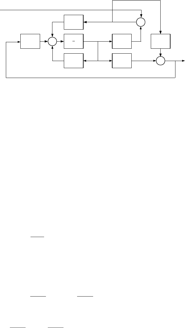
Fig. 8.25. State parametrised controller
8.7.4 Parametrisation of Transfer Functions of the Closed-Loop
System
The mathematical model of the closed-loop system in Fig. 8.23 can be written
as
u(s)
y(s)
=
A(s)(Y (s)+A(s)T(s)) A(s)(X(s) −B(s)T (s))
B(s)(Y (s)+A(s)T (s) B(s)(X(s) −B(s)T (s))
w(s)
d
u
(s)
(8.454)
Optimal control design for the controlled system with transfer function G(s)
can be performed in two steps. In the first a stabilising controller is found and
in the second a parameter T (s) is chosen such that the performance of the
closed-loop system is optimised. The cost function can be for example LQ.
This procedure will be explained in the following example.
Example 8.8:
Consider a first order controlled system with the transfer function
G(s)=
1
s +1
We want to find a stabilising controller for this system. Based on it, the
set of all stabilising controllers will be parametrised. Finally one controller
will be chosen that rejects asymptotically step disturbance.
Numerator and denominator of the process in fractional representation
can for example be given as
A(s)=
s +1
s + c
0
,B(s)=
1
s + c
0
where A(s),B(s) ∈ F
ps
. Equation (8.445) is of the form
s +1
s + c
0
X(s)+
1
s + c
0
Y (s)=1

372 8 Optimal Process Control
One particular solution is X(s)=1,Y (s)=c
0
− 1. This specifies one
stabilising controller. The set of all stabilising controllers is then of the
form
R(s)=
c
0
− 1+
s +1
s + c
0
T (s)
1 −
1
s + c
0
T (s)
The transfer function of the parametrised closed-loop system for input
variable d
u
and output variable e = −y is
G
ed
u
(s)=−B(s)(X(s) −B(s)T (s))
Substituting for B(s)=
1
s+c
0
and X(s) = 1 gives
G
ed
u
(s)=−
1
s + c
0
1 −
1
s + c
0
T (s)
=
−s −c
0
+ T(s)
(s + c
0
)
2
The final value theorem implies that the steady-state control error is zero
if
lim
s→0
G
ed
u
(s)=0
or if
T (s)=c
0
If this relation is substituted into the transfer function of the parametrised
controller then
R(s)=2c
0
− 1+
c
2
0
s
This is a PI controller with one design parameter. If c
0
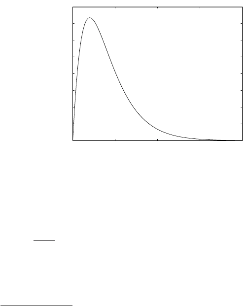
=0.5 then the
response to the unit step change of the disturbance is shown on Fig. 8.26.
8.7.5 Dual Parametrisation
It is not important from the parametrisation point of view which system in
the closed-loop system is parametrised. So far, the controller transfer function
was parametrised. If the controlled system is parametrised we speak about
the dual parametrisation.
Consider again the closed-loop system in Fig. 8.22. The controlled system
is described by transfer function
G(s)=
B(s)
A(s)
(8.455)
8.7 The Youla-Kuˇcera Parametrisation 373
0 5 10 15 20
0
0.1
0.2
0.3
0.4
0.5
0.6
0.7
0.8
t
y
Fig. 8.26. Closed-loop system response to the unit step disturbance on input
where B(s),A(s) ∈ F
ps
are coprime. This controlled system can be stabilised
by a controller with transfer function
R(s)=
Y (s)
X(s)
(8.456)
where Y (s),X(s) ∈ F
ps
are coprime. The set of all controlled systems sta-
bilised by the controller (8.456) is given as
B(s)+X(s)S(s)
A(s) −Y (s)S(s)
(8.457)
where S(s) ∈ F
ps
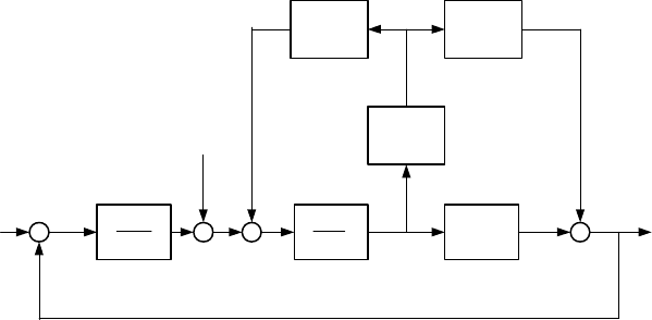
. The detailed block diagram of the parametrised controlled
system is given in Fig. 8.27.
Dual parametrisation is suitable for identification of the controlled system
in the closed-loop. Here, not the whole transfer function has to be identified.
Instead, only some deviation S(s) from nominal process can be estimated.
Moreover, the problem of estimation of S(s) represents only an open-loop
identification problem as
z(s)=S(s)x(s) (8.458)
and x(t), z(t) can be expressed in terms of u(t), y(t) that are measurable.
From Fig. 8.27 follows that u(s), y(s) are given as
u(s)=(A(s) −Y (s)S(s))x(s) (8.459)
y(s)=(B(s)+X(s)S(s))x(s) (8.460)
Multiplying (8.459) by X(s), (8.460) by Y (
s) and summing them gives
374 8 Optimal Process Control
e
)(sB
)(sX
)(
1
sA
)(sY
u
)(sS
−
w
u
d
y
)(
)(
sX
sY
z
x
Fig. 8.27. Parametrised controlled system in the closed-loop system
(A(s)X(s)+B(s)Y (s))x(s)=X(s)u(s)+Y (s)y(s) (8.461)
or
x(s)=X(s)u(s)+Y (s)y(s) (8.462)
From Fig. 8.27 also follows that
A(s)x(s)=u(s)+Y (s)z(s) (8.463)
B(s)x(s)=y(s) −X(s)z(s) (8.464)
Let us multiply (8.463) by
B(s), (8.464) by Y (s) and substract (8.464)
from (8.463). This yields
(A(s)X(s)+B(s)Y (s))z(s)=A(s)y(s) −B(s)y(s) (8.465)
or
z(s)=A(s)y(s) − B(s)y(s) (8.466)
The data needed for identification based on equation (8.458) are obtained
from (8.462) and (8.466).
We note that if both controller and plant are parametrised then the relation
between Youla-Kuˇcera parameters T (s), S(s) can significantly simplify the
control design problem.
8.7.6 Parametrisation of Stabilising Controllers for Multivariable
Systems
Matrices
˜
B
R
(s),
˜
A
R
(s) with elements in F
ps
(
˜
B
R
(s),
˜
A
R
(s) ∈ F
ps
) are rigth
coprime if

8.7 The Youla-Kuˇcera Parametrisation 375
˜
X
L
(s)
˜
A
R
(s)+
˜
Y
L
(s)
˜
B
R
(s)=I (8.467)
where
˜
Y
L
(s),
˜
X
L
(s) ∈ F
ps
. The left coprimeness of matrices
˜
A
L
(s)and
˜
B
L
(s) with matrix elements in F
ps
can be similarly defined.
The same procedure as for singlevariable systems can be performed to show
that the multivariable closed-loop system with structure given in Fig. 8.22 can
be parametrised to guarantee BIBO stability.
Consider a controlled system with a matrix transfer function
G(s)=
˜
A
−1
L
(s)
˜
B
L
(s)=
˜
B
R
(s)
˜
A
−1
R
(s) (8.468)
where
˜
A
L
(s),
˜
B
L
(s) ∈ F
ps
are left coprime and
˜
B
R
(s),
˜
A
R
(s) ∈ F
ps
are right
coprime. The set of all stabilising controllers is given as the matrix of transfer
functions
R(s)=(
˜
Y
R
(s)+
˜
A
R
(s)
˜
T (s))(
˜
X
R
(s) −
˜
B
R
(s)
˜
T (s))
−1
(8.469)
or
R(s)=(
˜
X
L
(s) −
˜
T (s)
˜
B
L
(s))
−1
(
˜
Y
L
(s)+
˜
T (s)
˜
A
L
(s)) (8.470)
where
˜
Y
L
(s),
˜
X
L
(s) ∈ F
ps
and
˜
Y
R
(s),
˜
X
R
(s) ∈ F
ps
are solution of the
equation
˜
A
L
(s) −
˜
B
L
(s)
˜
Y
L
(s)
˜
X
L
(s)
˜
X
R
(s)
˜
B
R
(s)
−
˜
Y
R
(s)
˜
A
R
(s)
= I (8.471)
The Youla-Kuˇcera parameter
˜
T (s) ∈ F
ps
has to be chosen such that
˜
X
L
(s) −
˜
T (s)
˜
B
L
(s)and
˜
X
R
(s) −
˜
B
R
(s)
˜
T (s) be non-singular.
8.7.7 Parametrisation of Stabilising Controllers for Discrete-Time
Systems
Parametrisation of controllers in the discrete-time domain has to take into
account some specific issues.
A system described by a proper rational transfer function F (z)isBIBO
stable if and only if it is Schur-stable. This implies that the transfer function
does not contain poles in the region |z|≥1.
To have a causal discrete-time closed-loop system and assuming proper
transfer function of the controller, the transfer function of the controlled sys-
tem has to be strictly proper. Stable rational functions in the z operator that
have all poles in the origin z = 0 are in fact polynomials in z
−1
.
Consider a transfer function of a discrete-time system of the form
G(z)=
b
0
z + b
1
z
2
+ a
1
z + a
2
(8.472)
376 8 Optimal Process Control
If we choose a stable denominator of the fractional representation as z
2
then
the transfer function can be written as
G(z)=
b
0
z
−1
+ b
1
z
−2
1+a
1
z
−1
+ a
2
z
−2
(8.473)
All relations for calculation of the parametrisation of all stabilising con-
trollers are the same for continuous and discrete-time systems. The difference
between them lies in the fact that continuous-time systems are represented by
stable fractions in s whereas discrete-time systems can be defined by polyno-
mials in z
−1
.
It can be shown that the optimal feedback control can be interpreted as the
pole placement design problem. From the nature of continuous-time systems
follows that the response of the closed-loop system to a step change in input
settles theoretically in infinity. The discrete-time control however, makes it
possible to force the output to follow the reference value in a finite time.
Dead-Beat Control
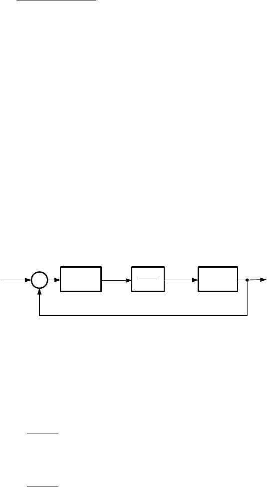
Consider the feedback closed-loop system shown in Fig. 8.28. The transfer
function of the controlled process is assumed to be strictly proper. We want
to design such a controller that the control error be zero after a finite time.
When it is found, the Youla-Kuˇcera parametrisation makes it possible to find
a set of such controllers and to choose among them the one that generates the
fastest response. Such a controller is called the dead-beat controller.
)(zR
e
u
y
−
w
)(zG
1
1
1
−
− z
Fig. 8.28. Discrete-time feedback closed-loop system
The controller consists of two parts in series. The first part with the trans-
fer function R(z) will be calculated by the control design, the second part is
fixed and guarantees the integrating properties of the controller.
The controlled process can be characterised by the fractional representa-
tion
G(z
−1
)=
B(z
−1
)
A(z
−1
)
(8.474)
Fractional representation of the controller is of the form
R(z
−1
)=
Q(z
−1
)
P (z
−1
)
(8.475)

8.7 The Youla-Kuˇcera Parametrisation 377
Integral part of the controller has been in the design procedure moved to the
controlled system G
I
= G/(1 − z
−1
). All poles of the closed-loop system are
placed in origin z = 0 for dead-beat control. The tracking error is given as
e(z
−1
)=
1
1+G
I
(z
−1
)R(z
−1
)
w(z
−1
) (8.476)
or
e(z
−1
)=(1− z
−1
)A(z
−1
)P (z
−1
)w(z
−1
) (8.477)
where
(1 −z
−1
)A(z
−1
)P (z
−1
)+B(z
−1
)Q(z
−1
) = 1 (8.478)
Transfer functions of all stabilising controllers are given as
R(z
−1
)=
Q(z
−1
)
P (z
−1
)
=
Y (z
−1
)+(1− z
−1
)A(z
−1
)T (z
−1
)
X(z
−1
) −B(z
−1
)T (z
−1
)
(8.479)
If reference sequence is given as a unit step change then
w(z
−1
)=
1
1 −z
−1
(8.480)
and the control error that is given as
e(z
−1
)=A(z
−1
)
X(z
−1
) −B(z
−1
)T (z
−1
)
(8.481)
is a polynomial. Equation (8.479) characterises a set of finite response con-
trollers with a parameter T (z
−1
).
The dead-beat controller that generates zero control error in the least
number of steps is obtained when
T (z
−1
) = 0 (8.482)
Example 8.9: The dead-beat controller for a continuous-time second order
www
system
Consider a continuous-time system with a transfer function
G(s)=
Z
2
(T
1
s + 1)(T
2
+1)
where Z
2
is the process gain and T
1
, T
2
are time constants. The transfer
function can be rewritten as
G(s)=
b
s0
(a
s2
s
2
+ a
s1
s +1)
where b
s0
= Z
2
, a
s2
= T
1
T
2
, a
s1
= T
1
+ T
2
.
The continuous-time system will be controlled by the feedback controller
(Fig.8.28). The controller R(z
−1
) has to guarantee

378 8 Optimal Process Control
1. finite time response of the closed-loop system,
2. finite time response of the closed-loop system in the minimum number
of steps.
The discretised transfer function of the controlled system is given in the
fractional representation as
G(z
−1
)=
b
1
z
−1
+ b
2
z
−2
1+a
I1
z
−1
+ a
I2
z
−2
where
b
1
= Z
2
−d
1
− d
2
−
T
1
(1 + d
2
)
T
2
− T
1
+
T
2
(1 + d
1
)
T
2
− T
1
b
2
= Z
2
d
1
+ d
2
+
T
1
d
2
T
2
− T
1
−
T
2
d
1
T
2
− T
1
d
1
=e
−
T
s
T
1
d
2
=e
−
T
s
T
2
a
I1
= −d
1
− d
2
a
I2
= d
1
d
2
and T
s
is the sampling period.
The discrete-time transfer function of the controlled system in series with
the discrete-time integrator is given as
G
i
(z
−1
)=
b
1
z
−1
+ b
2
z
−2
1+a
1
z
−1
+ a
2
z
−2
+ a
3
z
−3
where a
1
= a
I1
− 1, a
2
= a
I2
− a
I1
, a
3
= −a
I2
.
The minimum degree controller has the structure of the transfer function
given by (8.479) where polynomials
Y (z
−1
)=y
0
+ y
1
z
−1
+ y
2
z
−2
,X(z
−1
)=x
0
+ x
1
z
−1
are solution of the Diophantine equation
(1 + a
1
z
−1
+ a
2
z
−2
+ a
3
z
−3
)X(z
−1
)+(b
1
z
−1
+ b
2
z
−2
)Y (z
−1
)=1
If T (z
−1
)=t
0
then the controller with the transfer function
R(z
−1
)=
y
0
+ t
0
+(y
1
+ t
0
a
1
)z
−1
+(y
2
+ t
0
a
2
)z
−2
+ t
0
a
3
z
−3
x
0
+(x
1
− t
0
b
1
)z
−1
− t
0
b
2
z
−2
guarantees the finite-time response in four sampling steps.
If T (z
−1
) = 0, the controller with the transfer function
R(z
−1
)=
y
0
+ y
1
z
−1
+ y
2
z
−2
x
0
+ x
1
z
−1
guarantees finite-time response in a minimum time, i. e. in three sampling
steps.
MATLAB Program 8.2 implements the whole finite-time design for pa-
rameters Z
2
=2,T
1
=1,T
2
=2,T
s
=1andT (z
−1
)=−1.
8.7 The Youla-Kuˇcera Parametrisation 379
Program 8.2 (Calculation of the dead-beat controller)
(requires the Polynomial Toolbox for MATLAB)
z=2;t1=1;t2=2;ts=1;
G = tf(z, conv([t1 1],[t2 1]));
gz = c2d(G, ts);
zinteg = tf([1 0],[1 -1], ts);
% convert to Polynomial toolbox format manually
[b,a]=tfdata(gz, ’v’);
zii = [1; zi; zi^2];
b=b*[1;zi;zi^2];
a=a*[1;zi;zi^2];
a=a*(1-zi); % add integrator
%Design the DB controller
[x0,y0]=axbyc(a,b,1);
tt = -1;
x=x0-b*tt;
y=y0+a*tt;
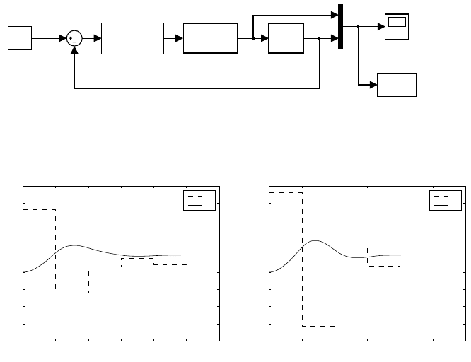
Fig. 8.29 shows the Simulink diagram using Program 8.2 for finite-time
control. Fig. 8.30a shows trajectories of the manipulated and controlled
variable of the continuous-time second order system with the finite-time
control design and for reference w(t)=1(t).
Fig. 8.30b shows trajectories of the manipulated and controlled variable
of the same system with the dead-beat control design.
We can notice that the non-zero parameter T (z
−1
) influences for example
magnitude of the manipulated variable. The price paid for it is a longer
duration of the closed-loop response. The minimum number of non-zero
values of the control error is 3, a constant T (z
−1
) gives one step more. The
same situation is for the manipulated variable where there are at least 4
non-zero values and one more for a constant T(z
−1
).
It is still possible for our second order system to find a dead-beat controller
that gives a faster response with smaller number of non-zero control error
values. This can be obtained using a two-degrees-of-freedom controller.
The minimum number of non-zero values of the control error is 2 and the
number of non-zero values of control increments is 3.
If the condition on finite number of control increment steps is relaxed to
a asymptotically stable sequence then it is possible for stable systems to
obtain the zero control error after one sampling step.
380 8 Optimal Process Control
data
To Workspace
Scope
G
Process
zinteg
Discrete
Integrator
Y(z^−1) / X(z^−1)
Controller
1
Constant
w
u
y
Fig. 8.29. Simulink diagram for finite-time tracking of a continuous-time second
order system
0 1 2 3 4 5 6
−4
−3
−2
−1
0
1
2
3
4
5
a
t
u,y
u
y
0 1 2 3 4 5 6
−4
−3
−2
−1
0
1
2
3
4
5
b
t
u,y
u
y
Fig. 8.30. Tracking in (a) finite (b) the least number of steps
8.8 LQ Control with Observer, State-Space
and Polynomial Interpretations
In Section 8.6 the state feedback control with observer was analysed and it is
shown in Fig. 8.13. One of the results is the separation theorem saying that
state feedback can be designed independently on the observer part.
Eigenvalues of the closed-loop system are composed of eigenvalues of the
matrix A − BK (state feedback without observer) and of eigenvalues of the
matrix A −LC. LQ control is then designed as follows:
1. LQ calculation of K,
2. design of L to guarantee stability,
3. state feedback control for singlevariable systems is implemented using the
control law
u = K ˆx (8.483)
Poles of the closed-loop system are determined by the poles of
o(s) = det (sI −(A − LC)) (8.484)
f(s) = det (sI −(A −BK)) (8.485)