Mikles J., Fikar M. Process Modelling, Identification, and Control

Подождите немного. Документ загружается.

8.12 Exercises 401

1. A feedback LQ controller with integrator based on state observation.

Choose Q = I in the cost function (8.488). Use the Polynomial toolbox

for MATLAB.

2. Implement the closed-loop system in Simulink.

Exercise 8.3:

Consider a controlled process with the transfer fuction

G(s)=

s + b

+ a

s + a

where b

=2,b

=0.1, b

=4,a

=3.

Find:

1. State-space representation of the controlled system.

2. Use the Polynomial toolbox for MATLAB and design a H

controller.

3. Implement the closed-loop system in Simulink and test it for various

choices of design parameters.

Exercise 8.4:

Consider a controlled process with the transfer fuction

G(s)=

s + b

+ a

s + a

where b

=2,b

=0.1, b

=4,a

=3.

Find:

1. State-space representation of the controlled system.

2. Use the Polynomial toolbox for MATLAB and design a H

controller with

integrator.

3. Implement the closed-loop system in Simulink and test it for various

choices of design parameters.

Predictive Control

This chapter deals with a popular control design method – predictive con-

trol. It explains its principles, features, and relations to other control meth-

ods. Compared to other parts of the book where continuous-time processes

are discussed, predictive control is mainly based on discrete-time or sampled

models. Therefore, derivations and expressions are presented mainly in the

discrete-time domain.

9.1 Introduction

Model Based Predictive Control (MBPC) or only Predictive Control is a broad

variety of control methods that comprise certain common ideas:

• a process model that is explicitly used to predict the process output for a

ﬁxed number of steps into future,

• a known future reference trajectory,

• calculation of a future control sequence minimising a certain objective

function (usually quadratic, that involves future process output errors and

control increments),

• receding strategy: at each sampling period only the ﬁrst control signal of

the sequence calculated is applied to a process controlled.

Among many useful features of MBPC, there is one that has created ex-

tensive industrial interest: the process constraints can easily be incorporated

into the method at the design stage.

MBPC algorithms are reported to be very versatile and robust in process

control applications. They usually outperform PID controllers and are applica-

ble to non-minimum phase, open-loop unstable, time delay, and multivariable

processes.

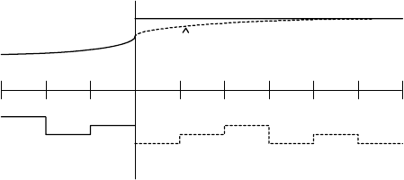
The principle of MBPC is shown in Fig. 9.1 and is as follows:

404 9 Predictive Control

k-1 k+1 k+2 k+N

Fig. 9.1. Principle of MBPC

1. The process model is used to predict the future outputs ˆy over some

horizon N. The predictions are calculated based on information up to

time k and on the future control actions that are to be determined.

2. The future control trajectory is calculated as a solution of an optimisa-

tion problem consisting of a cost function and possibly some constraints.

The cost function comprises future output predictions, future reference

trajectory, and future control actions.

3. Although the whole future control trajectory was calculated in the previ-

ous step, only its ﬁrst element u(k) is actually applied to the process. At

the next sampling time the procedure is repeated. This is known as the

Receding Horizon concept.

9.2 Ingredients of MBPC

9.2.1 Models

MBPC enables to plug-in directly any type of the process model. Of course,

linear models are most often used. This is caused by the possibility of an

analytic solution for the future control trajectory in unconstrained case.

The model should capture the process dynamics and to permit theoretical

analysis. The process model is required to calculate the predicted future out-

put trajectory. Some of the models incorporate directly disturbance model, in

others it is simply assumed that disturbance is constant.

Impulse Response

The theoretical impulse sequence is usually truncated for practical reasons.

The output is related to the input by the equation

y(k)=



i=1

u(k − i)=H(q

−1

)u(k) (9.1)

9.2 Ingredients of MBPC 405

where H(q

−1

)=h

−1

+ h

−2

+ ···h

−N

and q

−1

is the backward shift

operator deﬁned as y(k)q

−1

= y(k −1).

The drawbacks of this model are:

• high value of N needed ≈ 50,

• only stable processes can be represented.

Step Response

The step response model is very similar to the FIR model with the same

drawbacks. Again, truncated step response is used for stable systems

y(k)=



i=1

Δu(k − i)=G(q

−1

)(1 −q

−1

)u(k) (9.2)

As the step and impulse responses are easily collected, the methods based on

them gained large popularity in the industry. The step model is for example

used in DMC.

Transfer Function

This model is used in GPC, EHAC, EPSAC, and others. The output is mod-

elled by the equation

A(q

−1

)y(k)=B(q

−1

)u(k) (9.3)

The advantage of this representation is that it is also valid for unstable models.

On the other side, order of the A, B polynomials is needed.

State Space

The representation of the state-space model is as follows:

x(k +1)=Ax(k)+Bu(k) (9.4)

y(k)=Cx(k) (9.5)

Its advantage is an uncomplicated way of dealing with multivariable processes.

However, the state observer is often needed.

Others

As it was stated before, any other process model is acceptable. Continuous

nonlinear models in the form of ordinary diﬀerential equations are often used.

Their drawbacks are large simulation times. The area of dynamic optimisation

usually covers them.

Recently, neural and fuzzy models have gained popularity. Two approaches

have emerged. The model is either directly used, or it only generates some

process characteristics: step or impulse responses.

406 9 Predictive Control

Disturbances

The most general disturbance model is an ARMA process (c. f. page 223)

given by

n(k)=

C(q

−1

)

D(q

−1

)

ξ(k) (9.6)

with ξ(k) being white noise. Within the MBPC framework, the D = ΔA

polynomial includes the integrator Δ =1−q

−1

to cover random-walk distur-

bances. Another pleasing property of the integrator is the set-point tracking

(integral action).

When the process model of the form (9.3) is used, the overall model is

then called CARIMA (or ARIMAX) and is given as

ΔAy(k)=BΔu(k)+Cξ(k) (9.7)

9.2.2 Cost Function

The standard cost function used in predictive control contains quadratic terms

of (possibly ﬁltered) control error and control increments on a ﬁnite horizon

into the future

I =



i=N

[P ˆy(k + i) − w(k + i)]

+ λ



i=1

[Δu(k + i − 1)]

(9.8)

where ˆy(k + i) is the process output of i steps in the future predicted on the

base of information available upon the time k, w(k + i) is the sequence of

the setpoint variable and Δu(k + i − 1) is the sequence of the future control

increments that have to be calculated.

Implicit constraints on Δu are placed between N

and N

Δu(k + i − 1) = 0,N

<i≤ N

(9.9)

The cost function parameters are following:

• Horizons N

, N

,andN

are called minimum, maximum, and control hori-

zon, respectively. The horizons N

and N

mark the future time interval

where it is desirable to follow the reference trajectory. N

should be at least

equal to T

+ 1 where T

is the assumed value of the process time delay.

Also, the non-minimum phase behaviour of the process can be eliminated

from the cost by letting N

to be suﬃciently large. The value of N

should

cover the important part of the step response curve, it is usually chosen

to be about the settling time of the plant T

(see page 257). The use of

the control horizon N

reduces the computational load of the method.

9.3 Derivation and Implementation of Predictive Control 407

• Reference trajectory w(k + i) is assumed to be known beforehand. If it is

not the case, several approaches are possible. The simplest way is to assume

that the future reference is constant and equal to the desired setpoint w

∞

The preferred approach is to use smooth reference trajectory that begins

from the actual output value and approaches asymptotically via the ﬁrst

order ﬁlter the desired setpoint w

∞

. It is thus given as

w(k)=y(k) (9.10)

w(k + i)=αw(k + i − 1) + (1 −α)w

∞

(9.11)

The parameter α determines smoothness of the trajectory with α → 0

being the fastest and α → 1 being the slowest trajectory.

The same eﬀect can be achieved with the use of the ﬁlter polynomial

P (z

−1

). The output y follows the model trajectory

w. The corresponding

ﬁlter to the previous ﬁrst order trajectory is given as

P (z

−1

1 −αz

−1

1 −α

(9.12)

9.3 Derivation and Implementation of Predictive Control

In this part, Generalised Predictive Control (GPC) will be derived. The GPC

method is in the principle applicable to both SISO and MIMO processes and

is based on input-output models. We begin the derivation for SISO systems for

simplicity and show in the actual implementation of the method, how to treat

MIMO systems. Alternatively, the predictor equations will also be derived for

state-space models.

9.3.1 Derivation of the Predictor

The ﬁrst step in the development of MBPC is derivation of the optimal pre-

dictor. We start with the CARIMA model (9.7) of the form

A(q

−1

)y(k)=B(q

−1

)u(k − 1) +

C(q

−1

)

ξ(k) (9.13)

Note that we use explicitly u(k −1) and thus the polynomial B has a non-zero

absolute coeﬃcient. We use u(k −1) because u(k) will constitute one element

of the optimised variables.

Now let us think about this equation j steps in the future. This is accom-

plished by multiplication of this equation by q

and it yields

y(t + j)=

u(t + j − 1) +

ΔA

ξ(t + j) (9.14)

The last term of this equation contains past and future values of ξ.Wemay

separate them by performing long division on the term C/(ΔA) and by sep-

arating the ﬁrst j terms (quotient) with positive powers of q. This yields

408 9 Predictive Control

C(q

−1

)

ΔA(q

−1

)

= E

−1

)+q

−j

−1

)

ΔA(q

−1

)

(9.15)

where the polynomial E

has degree j − 1. Inserting back into (9.14) gives

y(t + j)=

u(t + j − 1) + E

ξ(t + j)+

ΔA

ξ(k) (9.16)

The last term contains actual value of the disturbance ξ(k). This can be

calculated from (9.13) and inserted back into the last equation

y(t + j)=

u(t + j − 1) −

ΔAC

Δu(k − 1) +

y(k)+E

ξ(t + j)



ΔA

− q

−j

ΔAC



Δu(t + j − 1) +

y(k)+E

ξ(t + j)



ΔA

− q

−j

ΔA



Δu(t + j − 1) +

y(k)+E

ξ(t + j)(9.17)

and ﬁnally substituting (9.15) into the term containing Δu(t + j − 1) yields

y(t + j)=

Δu(t + j − 1) +

y(k)+E

ξ(t + j) (9.18)

Again, we separate unknown (future and present) control actions from the

known (past) ones by the means of the polynomial division

B(q

−1

)

C(q

−1

)

= G

−1

)+q

−j

−1

)

C(q

−1

)

(9.19)

This gives the ﬁnal form for the future value of the system output

y(t + j)=G

Δu(t + j − 1) +

Δu(k − 1) +

y(k)+E

ξ(t + j) (9.20)

It is obvious that the minimum variance prediction of y(t+j) for given data up

to time k is obtained by replacing the last term containing future disturbances

by zero and yields

ˆy(t + j)=G

Δu(t + j − 1) +

Δu(k − 1) +

y(k) (9.21)

ˆy(t + j)=G

Δu(t + j − 1) + y

(t + j) (9.22)

Thus, to obtain the j step predictor, two polynomial divisions (or equiva-

lently Diophantine equations) are to be solved

C = E

ΔA + q

−j

(9.23)

= G

C + q

−j

(9.24)

To implement calculation of the predictor eﬃciently, it is necessary to

understand correctly the rˆole of the equation (9.22) and the terms involved

in it.

9.3 Derivation and Implementation of Predictive Control 409

Let us ﬁrst assume that all future control increments are zero. Equa-

tion (9.22) gives

ˆy(t + j)=y

(t + j) (9.25)

Hence, the term y

can be determined by the free response of the system if

the input remains to be constant at the last computed value u(k − 1).

Similarly, let us assume that the system is at the time k in the steady-state

and we may assume without loss of generality that the steady-state is zero.

This gives a zero free response y

(t + j). If at time k the system is subject to

unit step in input, the system output is given from (9.22) as

ˆy(t + j)=G

−1

)Δu(t + j − 1)

= g

Δu(t + j − 1) + g

Δu(t + j − 2) + ···+ g

j,j−1

Δu(k)

= g

j,j−1

(9.26)

Thus, the polynomial G

−1

) contains the system step response coeﬃcients.

As an alternative way to show this consider (9.15) multiplied by B/C:

ΔA

+ q

−j

ΔAC

= G

+ q

−j

+ q

−j

ΔAC

(9.27)

which shows that G

is the quotient of the division B/(ΔA).

9.3.2 Calculation of the Optimal Control

The GPC cost function is given by (9.8). Let us now assume for simplicity

that N

=1,N

= N

,P = 1. It follows that all output prediction up to time

t + N

are needed. Let us stack individual output predictions, future control

increments, future reference trajectory, and free responses into corresponding

vectors

ˆy

=[ˆy(t +1), ˆy(t +2),...,ˆy(t + N

)] (9.28)

=[y

(t +1),y

(t +2),...,y

(t + N

)] (9.29)

˜u

=[Δu(k), Δu(t +1),,...,Δu(t + N

− 1)] (9.30)

=[w(t +1),w(t +2),...,w(t + N

)] (9.31)

(9.32)

To vectorise the predictor (9.22), let us form a matrix containing step response

coeﬃcients given as

G =

⎛

⎜

⎝

0 ... ... 0

0 ... 0

. g

−1

... ... g

⎞

⎟

⎠

(9.33)

410 9 Predictive Control

If we take into eﬀect the real value of N

, then the ﬁrst N

− 1rowsofthe

matrix G should be removed. Similarly, only the ﬁrst N

columns are retained.

Thus, the real matrix G has the dimension [N

− N

+1× N

Hence, the predictor in the vector notation can be written as

ˆy = G˜u + y

(9.34)

and the cost function (9.8) as

I =(ˆy −w)

(ˆy − w)+λ˜u

˜u

=(G˜u + y

− w)

(G˜u + y

− w)+λ˜u

˜u

= c

+2g

˜u + ˜u

H ˜u (9.35)

where the gradient g and Hessian H are deﬁned as

= G

− w) (9.36)

H = G

G + λI (9.37)

Minimisation of the cost function 9.35 now becomes a direct problem of

linear algebra. The solution in the unconstrained case can be found by setting

partial derivative of I with respect to ˜u to zero and yields

˜u = −H

−1

g (9.38)

This equation gives the whole trajectory of the future control increments

and as such it is an open-loop strategy. To close the loop, only the ﬁrst element

of ˜u,e.g.Δu(k) is applied to the system and the whole algorithm is recom-

puted at time t + 1. This strategy is called the Receding Horizon Principle

and is one of the key issues in the MBPC concept.

If we denote the ﬁrst row of the matrix (G

G + λI)

−1

by K then the

actual control increment can be calculated as

Δu(k)=K(w − y

) (9.39)

Hence, if there is no diﬀerence between the free response and the setpoint

sequence in the future, the actual control increment will be zero. If there

will be some diﬀerences in the future, the actual control increment will be

proportional to them with the factor K.

To summarise the procedure, it should be noticed, that only two plant

characteristics are needed: free response y

that is changing at each sampling

time and step response G(z

−1

) which is in the case of time invariant sys-

tem needed only once. Moreover, also the Hessian matrix H that should be

inverted, contains only information from the step response and can also be

calculated beforehand. The calculation of the actual control increment is thus

dependent only on weighted sum of past inputs and outputs contained in y

and forms therefore a linear control law.

9.3 Derivation and Implementation of Predictive Control 411

9.3.3 Closed-Loop Relations

It follows from (9.39) that the control is a linear combination of the setpoint

and free response. As the control law and the controlled process are linear, it is

possible to derive the characteristic equation and the poles of the closed-loop

system.

The equation (9.39) can be written in the time domain

Δu(k)=



j=N

(w(t + j) −y

(t + j)) (9.40)

Using the free response from (9.22) yields

Δu(k)=



j=N



w(t + j) −

−1

Δu(k) −

y(k)



(9.41)

CΔu(k)=C



j=N

w(t + j) −



j=N

−1

Δu(k) −



j=N

y(k)(9.42)

⎛

⎝

C + q

−1



j=N

⎞

⎠

Δu(k)=C



j=N

w(t + j) −



j=N

y(k) (9.43)

Let us assume for simplicity that the future setpoint change is constant,

i. e. w(t + j)=w(k). The control law constitutes a two degree-of-freedom

(2DoF) controller

Δu(k)=R

w(k) −P

y(k) (9.44)

where

C + q

−1

j=N

(9.45)

= C (9.46)

j=N

(9.47)

To derive the characteristic equation of the closed-loop systems, the control

law is inserted into the CARIMA model (9.13)

AΔy(k)=Bq

−1



w(k) −

y(k)



+ Cξ(k) (9.48)

y(z)=

−1

AΔ + P

−1

w(z)+

AΔ + P

−1

ξ(z) (9.49)

The denominator polynomial is the characteristic equation. Its further manip-

ulation gives