Mikles J., Fikar M. Process Modelling, Identification, and Control

Подождите немного. Документ загружается.

8.8 Observer LQ Control, State-Space and Polynomial Interpretations 381

Based on the results in the state-space domain we will now derive LQ control

in the polynomial domain.

8.8.1 Polynomial LQ Control Design with Observer

for Singlevariable Systems

Consider a linear reachable and observable singlevariable system

˙x(t)=Ax(t)+Bu(t), x(0) = x

(8.486)

y(t)=Cx(t) (8.487)

and a cost function

I =



∞



(t)Qx(t)+u

(t)



dt (8.488)

where Q is a real symmetric positive semideﬁnite matrix. LQ control prob-

lem consists in ﬁnding a control law (u = function(x)) such that guarantees

asymptotic stability of the closed-loop system and minimisation of I for any

As it was shown in Section 8.2, the control law is of the form

u = −Kx (8.489)

where

K = B

P (8.490)

and P is a symmetric positive semideﬁnite solution of the matrix Riccati

equation

PA+ A

P − PBB

P = −Q (8.491)

Deterministic state estimate is given as

ˆx(t)=Aˆx(t)+Bu(t)+L (y(t) − C ˆx) , ˆx(0) = ˆx

(8.492)

Matrix L is chosen in such a way that the estimation error

e(t)=x(t) − ˆx(t) (8.493)

with initial condition

e(0) = x

− ˆx

(8.494)

asymptotically converges to origin.

Control law (8.489) cannot directly be used. It was shown in Section 8.6

that polynomial implementation of the observer gives the control law of the

form

382 8 Optimal Process Control

u =˜u (8.495)

where

˜u = −K ˆx (8.496)

Polynomial solution of the deterministic control design with controller input

being y can be obtained as a combination of polynomial controller and ob-

server.

Theorem 8.5 (LQ control with observer). Consider a reachable and

observable singlevariable system

˙x(t)=Ax(t)+Bu(t), x(0) = x

(8.497)

y(t)=Cx(t) (8.498)

where

(sI −A)

−1

B =

(s)

a(s)

(8.499)

C (sI − A)

−1

B =

b(s)

a(s)

(8.500)

and where a(s) is the characteristic polynomial of the matrix A and polyno-

mials a(s), b(s) are coprime.

The control law based on state estimation and minimising the cost function

I is given as

u = −

q(s)

p(s)

y (8.501)

where polynomials p(s), q(s) are a solution of the equation

a(s)p(s)+b(s)q(s)=o(s)f(s) (8.502)

Polynomial p(s) is of degree n if stable polynomial o(s) is of degree n (full

order observer case), or is of degree n −1 is stable polynomial o(s) is of degree

n −1 (reduced order observer case). Polynomial q(s) is of degree n −1. Stable

monic polynomial f(s) is deﬁned as

a(−s)a(s)+B

(−s)QB

(s)=f(−s)f(s) (8.503)

Proof. The proof of Theorem 8.3 shows that the characteristic polynomial

f(s) of the closed-loop matrix A −BK and the controller gain K satisfy the

following relation

a(s)+KB

(s)=f(s) (8.504)

where the stable monic polynomial f(s) is solution of spectral factorisation

equation (8.503). If f (s) exists, it is unique. Matrix K from (8.504) is also

solution of the Riccati equation

8.8 Observer LQ Control, State-Space and Polynomial Interpretations 383

PA+ A

P − PBB

P = −Q + sP − sP (8.505)

This equation can be manipulated as follows



−sI −A



P + P (sI − A)=Q −PBB

P (8.506)



−sI −A



−1



−sI −A



P (sI − A)

−1

+ B



−sI −A



−1

P (sI − A)(sI −A)

−1

= B



−sI −A



−1



Q −PBB



(sI −A)

−1

B (8.507)

P (sI − A)

−1

B + B



−sI −A



−1

= B



−sI −A



−1



Q −PBB



(sI −A)

−1

B (8.508)

As (8.499) holds, equation (8.508) can be written as

(s)a(−s)+B

(−s)PBa(s)=B

(−s)



Q −PBB



(8.509)

(s)a(−s)+B

(−s) K

a(s)

= B

(−s)QB

(s) − B

(−s) K

(s) (8.510)

a(−s)a(s)+B

(−s)K

a(s)+KB

(s)a(−s)+B

(−s)K

(s)

= a(−s)a(s)+B

(−s)QB

(s) (8.511)



a(−s)+B

(−s) K



(a(s)+KB

(s))

= a(−s)a(s)+B

(−s)QB

(s) (8.512)

Considering (8.504) shows that (8.512) is the same as (8.503) which proves

one part of the theorem.

The proof of Theorem 8.3 also gives equation of the asymptotic ob-

server (8.310) where polynomials on this equation are solution of (8.320).

Substituting K ˆx from (8.310) into (8.496) yields

u = −

r(s)

o(s)

u −

q(s)

o(s)

y (8.513)

p(s)=o(s)+r(s) (8.514)

then (8.513) is of the form (8.501). As (8.302), (8.317), (8.514) hold, equa-

tion (8.310) can be transformed into (8.502). This concludes the proof. 

384 8 Optimal Process Control

Example 8.10:

Consider a controlled process with transfer function of the form

G(s)=

s + a

The objective is to ﬁnd for this system the transfer function of the feedback

LQ controller with state observer. It is required that the controller contains

an integration term. Therefore, we consider in the cost function (8.488)

derivative ˙u(t)inplaceofu(t) and the weighting matrix Q is reduced to

Q = Q

From Theorem 8.5 follows that the controller transfer function is in our

case given as

R(s)=

+ q

s(p

s + p

)

where

= o

+ f

− a

+ f

− a

are solutions of the Diophantine equation

(s + a

)s(p

s + p

)+b

s + q

)=o(s)f(s)

and

o(s)=s + o

is a stable monic polynomial. Coeﬃcients of the stable monic polynomial

f(s)=s

+ f

s + f

follow from the spectral factorisation equation

(−s + a

)(−s)(s + a

)s +



−b









= f(−s)f (s)

and are given as

= b



+2f

The observer polynomial o(s) can be suitably chosen according to further

requirements on control performance.

8.8 Observer LQ Control, State-Space and Polynomial Interpretations 385

8.8.2 Polynomial LQ Design with State Estimation

for Multivariable Systems

Consider a controllable and observable multivariable system

˙x(t)=Ax(t)+Bu(t), x(0) = x

(8.515)

y(t)=Cx(t) (8.516)

and a cost function

I =



∞

(t)Qx(t)+u

(t)u(t))dt (8.517)

LQ control law is implemented as

u(t)=−K ˆx(t) (8.518)

where

K = B

P (8.519)

and P is a symmetric positive semideﬁnite solution of the algebraic Riccati

equation

PA+ A

P − PBB

P = −Q (8.520)

Deterministic state estimate is given as

˙x(t)=Aˆx(t)+Bu(t)+L(y(t) −C ˆx(t)) , ˆx(0) = x

(8.521)

As (8.398) holds then

K = X

−1

(8.522)

where X

, Y

are a solution of the Diophantine equation

(s)+Y

(s)=F

(s) (8.523)

This was derived in polynomial design of pole placement controllers for multi-

variable systems. LQ control can be interpreted as the pole placement design.

This implies that we need to determine a matrix F

(s) such that LQ cost

function is minimised. To ﬁnd such a matrix, we will transform the Riccati

equation as follows.

Adding sP to either side of equation (8.520) gives



−sI −A



P + P (sI − A)=Q −PBB

P (8.524)

Multiplying from the left by B

(−sI −A

)

−1

, from the right by (sI −A)

−1

and using (8.522), (8.398) gives

386 8 Optimal Process Control

(−s)K

(s)+A

(−s)KB

(s)+B

(−s)K

(s)

= B

(−s)QB

(s) (8.525)

Adding A

(−s)A

(s) to either side of equation yields

(−s)+B

(−s)K

)(A

(s)+KB

(s))

= A

(−s)A

(s)+B

(−s)QB

(s) (8.526)

From (8.405) follows that LQ design F

(s) needed for determination of K

from (8.523) is a solution of the spectral factorisation equation

(−s)F

(s)=A

(−s)A

(s)+B

(−s)QB

(s) (8.527)

All subsequent steps of the multivariable LQ control design are the same as

in the pole placement design. Thus, L is determined from (8.411) and the

controller transfer function matrix from (8.413).

Example 8.11: Multivariable LQ control

www

Consider a continuous-time multivariable controlled system with the

transfer function matrix

G(s)=A

−1

(s)B

(s)

where

(s)=



1+0.3s 0.5s

0.1s 1+0.7s



, B

(s)=



0.20.4

0.60.8



The task is to design LQ controller with observer. It is required that the

controller contains an integration term.

The problem can be solved using the relations given above and it is shown

in Program 8.3. We use the Polynomial toolbox for MATLAB.

Program 8.3 (LQ controller design – optlq22.m)

%PLANT

al = [1+.3*s, .5*s; .1*s 1+0.7*s];

bl = [.2 .4;.6 .8];

bl = pol(bl);

[a,b,c,d] = lmf2ss(bl,al);

G = ss(a,b,c,d);

%CONTROLLER

als = al*s;

[As,Bs,Cs,Ds] = lmf2ss(bl,als);

[Brs,Ar] = ss2rmf(As,Bs,eye(4));

Q =10*eye(4);

Fr = spf(Ar’*Ar+Brs’*Q*Brs);

8.8 Observer LQ Control, State-Space and Polynomial Interpretations 387

[Xl,Yl] = xaybc(Ar,Brs,Fr);

K=mldivide(Xl,Yl);

K=lcoef(K);

[Bls,Al] = ss2lmf(As,eye(4),Cs);

%V=10*eye(4);

%Ol = spf(Al*Al’+Bls*V*Bls’);

Ol =[-3.1-3.4*s-0.18*s^2 -0.5-0.58*s-0.011*s^2;

-0.5-0.62*s-0.055*s^2 3.1+4*s+0.9*s^2];

[Xr,Yr] = axbyc(Al,Bls,Ol);

L=mrdivide(Yr,Xr);

L=lcoef(L);

acp = As-L*Cs-Bs*K;

bcp = L;

ccp = K;

dcp = zeros(2);

[brp,arp]=ss2rmf(acp,bcp,ccp,dcp);

[ac,bc,cc,dc] = rmf2ss(brp,arp*s)

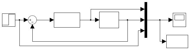
The closed-loop system is implemented in Simulink scheme optlq22s.mdl

shown in Fig. 8.31.

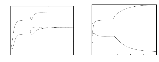
Fig. 8.32a,b shows trajectories of input and output variables of the con-

trolled process.

To Workspace

data

Step

Scope

Process

Controller

x’ = Ax+Bu

y = Cx+Du

w yu

Fig. 8.31. Scheme optlq22s.mdl in Simulink for multivariable continuous-time LQ

control

Note 8.6. Program 8.3 describes MIMO LQ control design. However, it is writ-

tentobeusedinPA,LQG,orH

control.

If pole assignment is desired, we comment the line in the program that

computes spectral factorisation of the matrix F

Fr = spf(Ar’*Ar+Brs’*Q*Brs)

388 8 Optimal Process Control

0 5 10 15 20 25

−0.5

0.5

1.5

2.5

(a)

y,w

0 5 10 15 20 25

−3

−2

−1

(b)

Fig. 8.32. Trajectories of (a) output, and setpoint variables, (b) input variables of

the multivariable continuous-time process controlled with LQ controller

and substitute it with a corresponding matrix of appropriate dimensions that

places the feedback poles.

To calculate LQG controller (see Section 8.9.2), we uncomment lines with

the second spectral factorisation equation

V=10*eye(4)

Ol = spf(Al*Al’+Bls*V*Bls’)

controller can be implemented similarly if diﬀerences between right

hand sides of Riccati equations (8.539), (8.576), (8.607), and (8.609) are taken

into account.

8.9 LQG Control, State-Space and Polynomial

Interpretation

Based on the state LQG control with the Kalman ﬁlter we will derive expres-

sions for polynomial LQG systems for both singlevariable and multivariable

systems.

8.9.1 Singlevariable Polynomial LQG Control Design

Consider a linear singlevariable controllable and observable system

˙x(t)=Ax(t)+Bu(t)+ξ

(t) (8.528)

y(t)=Cx(t)+ξ(t) (8.529)

where ξ

(t) is a random vector process with normal distribution and

E {ξ

(t)} = 0 (8.530)



(t)ξ

(τ)



= V δ (t − τ) , V ≥ 0 (8.531)

8.9 LQG Control, State-Space and Polynomial Interpretation 389

ξ(t) a random vector process with normal distribution and with

E {ξ(t)} = 0 (8.532)

E {ξ(t)ξ (τ )} = δ (t − τ) , (8.533)

We assume thatξ

(t)andξ(t) are uncorrelated in time.

Linear Quadratic Gaussian (LQG) problem consists in ﬁnding a control

law (u = function(x)) such that asymptotic stability of the closed-loop system

is guaranteed and the cost function I is minimised where

I = E

⎧

⎪

⎨

⎪

⎩

lim

→−∞

→∞

− t





(t)Qx(t)+u

(t)



⎫

⎪

⎬

⎪

⎭

(8.534)

and Q is a real symmetric positive semideﬁnite matrix.

The separation theorem says that it is possible to solve LQG problem by

solving the deterministic LQ problem at ﬁrst

˙x(t)=Ax(t)+Bu(t) (8.535)

with the cost function

I =



∞



(t)Qx(t)+u

(t)



dt (8.536)

This results in a control law of the form

u(t)=−Kx(t) (8.537)

where

K = B

P (8.538)

and P is a symmetric positive semideﬁnite solution (P

= P ≥ 0)ofthe

algebraic Riccati equation

PA+ A

P − PBB

P = −Q (8.539)

In the second step, the state ˆx of the system (8.528), (8.529) is estimated

using the Kalman ﬁlter

ˆx(t)=Aˆx(t)+Bu(t)+L (y(t) − C ˆx(t)) (8.540)

where

L = NC

(8.541)

and N is a symmetric positive semideﬁnite solution (N

= N ≥ 0)ofthe

algebraic Riccati equation

390 8 Optimal Process Control

AN + NA

− NC

CN = −V (8.542)

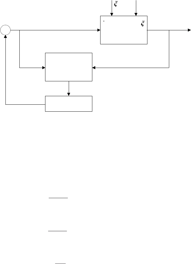
Finally, the control law is implemented as

u(t)=−K ˆx(t) (8.543)

The LQG control is illustrated in Fig. 8.33.

++=

Cxy

BuAxx

Kalman filter

Fig. 8.33. Block diagram of LQG control

Theorem 8.7 (LQG control). Consider a controllable and observable sin-

glevariable system

˙x(t)=Ax(t)+Bu(t)+ξ

(t) (8.544)

y(t)=Cx(t)+ξ(t) (8.545)

where

(sI −A)

−1

B =

(s)

a(s)

(8.546)

a(s), B

(s) are right coprime for a reachable system,

C (sI − A)

−1

(s)

a(s)

(8.547)

a(s), B

(s) are left coprime for an observable system,

C (sI − A)

−1

B =

b(s)

a(s)

(8.548)