Mikles J., Fikar M. Process Modelling, Identification, and Control

Подождите немного. Документ загружается.

432 9 Predictive Control

−1 −0.5 0 0.5 1

−1

−0.5

0.5

u = −0.52 x

−0.94 x

u = −1

u = 1

Fig. 9.3. Controller regions and the optimal control for the double integrator

example

2. If the sampling time has not yet been speciﬁed, select it as the larger value

that satisﬁes

≤ 0.1T, T

≤ 0.5T

(9.124)

3. Calculate the discrete dead time

(rounded to the next integer)

= T

+ 1 (9.125)

4. Set N

=1,and

=5T/T

(9.126)

5. Select the control horizon N

(usually between 1–6) and calculate the

control weighting λ as

f =

0 N

500



3.5T

+2−

−1



> 1

(9.127)

λ = fZ

(9.128)

9.7.2 Multivariable Tuning based on the First Order Model

This tuning strategy is a generalisation of the previous approach to multivari-

able systems with R outputs and S inputs. Again, it is based on the analysis

of the ﬁrst order system with time delay.

9.7 Tuning 433

1. Approximate the process dynamics of all controller output-process vari-

able pairs with ﬁrst order plus dead time models:

(s)

s +1

−T

d,rs

(9.129)

2. Select the sampling time as close as possible to:

= max(0.1T

, 0.5T

d,rs

),T

= min(T

) (9.130)

3. Set N

= 1, compute the prediction horizon N

= max



+ k



d,rs

+ 1 (9.131)

4. Select a control horizon N

, equal to 63.2% of the settling time of the

slowest sub-process in the multivariable system:

= max



+ k



(9.132)

5. Select the controlled variable weights γ

, to scale process variable mea-

surements to similar magnitudes

6. Compute the control weightings λ

500



r=1





− k

−

+2−

M − 1



(9.133)

Fine tuning of the method is performed by increasing the corresponding γ

of the process variable for which tighter control is desired and increasing the

corresponding λ

of the manipulated variable for which less aggressive moves

are desired.

9.7.3 Output Horizon Tuning

This tuning strategy assumes the active tuning parameter to be the output

horizon N

with all other ﬁxed at the values

=1,N

=1,P=1,λ= 0 (9.134)

It is well known that if N

→∞, mean-level controller results. This controller

is rather conservative as its speed is the same as step responses.

The other limit for N

is the value of the process dead time. If N

= T

+1,

where T

represents process dead time, then we have the Minimum Variance

(MV) controller known to be unstable for non-minimum phase plants.

The practical range for N

can be speciﬁed as

+1<N

≤ T

(9.135)

434 9 Predictive Control

where T

is the time when process reaches about 90% of its ﬁnal value after

input step change and T

is the sampling time.

If the process is uncertain, it is better to start with a larger value of N

The minimum value of N

for non-minimum phase plants should be such that

has the same sign as the process gain.

9.7.4 λ Tuning

In this case the active tuning parameter is the penalisation of control moves

λ. All other parameters are ﬁxed as

= deg(B)+1,N

= deg(A)+1,N

≥ N

+ N

− 1 ≈ t

,P=1

(9.136)

With λ equal to zero, dead-beat controller results. This is too rapid in the

majority of cases. Hence, with increasing value of λ the controller is made

more conservative. It might be shown that the closed-loop poles converge to

the open loop poles if λ →∞.Thusλ tuning is not recommended for unstable

plants.

It has been found that to desensitise the closed-loop system to changes in

process dynamics, the actual λ should be proportional to B(1)

λ = λ

B(1)

(9.137)

with λ

being a constant.

To determine a starting value of λ, the following relation can be used:

λ =

m tr(G

(9.138)

and m is a factor of detuning the controller relative to the dead-beat control.

The control increments are approximately reduced by a factor m+1 compared

to that of the dead-beat strategy.

From this starting value of λ, an initial guess for λ

can be determined

from (9.137).

9.7.5 Tuning based on Model Following

As it has been shown before, the P polynomial can be used to generate ref-

erence trajectory w/P. GPC can be set up to follow this trajectory exactly

and so to place the closed-loop poles at the process zeros. In order to have a

more practical controller, the model following can be detuned. This may be

accomplished by either increasing N

or λ.

The ﬁxed parameters are as follows:

=1,N

= deg(A)+1,N

≥ N

+ T

≈ t

,λ= 0 (9.139)

9.7 Tuning 435

Most often, the models M =1/P are of the ﬁrst and the second order. If

the ﬁrst order closed-loop model is assumed to be of the form

M(s)=

Ts+1

(9.140)

then its discrete equivalent is

M(z

−1

(1 −p

−1

1 −p

−1

(9.141)

where p

=exp(−T

/T ). The polynomial P can thus be chosen as (cf. equa-

tion (9.12)) and P (1) is equal to 1 to ensure the oﬀset-free behaviour. This

model is applicable mainly for simpler plants as the ﬁrst order trajectory may

sometimes generate excessive control actions.

The second order model can be of the form

M(s)=

+2Tζs+1

(9.142)

Its discrete time equivalent is

M(z

−1

+ n

−2

1+p

−1

+ p

−2

(9.143)

where

= −2exp



−ζT



cos







1 −ζ



(9.144)

=exp



−2ζT



(9.145)

Ignoring the numerator dynamics, the polynomial P may be speciﬁed as

P (z

−1

1+p

−1

+ p

−2

1+p

+ p

(9.146)

The dominant time constant of the closed-loop system is approximately 2T

and the fractional overshoot is solely a function of the damping factor ζ:

=exp

−πζ



1 −ζ

(9.147)

and thus the user can then specify the desired rise time and overshoot and

translate these settings into an appropriate P polynomial.

9.7.6 The C polynomial

The CARIMA model includes knowledge about the disturbance properties in

the polynomial C. This can be estimated on-line using a suitable recursive

436 9 Predictive Control

identiﬁcation algorithm. However, this is rather diﬃcult in practice, because

the convergence of the C polynomial coeﬃcients is rather slow.

Therefore, a more realistic approach is to set C by user directly. The value

that has been suggested as a default in the literature is of the form

C =(1− 0.8z

−1

)

(9.148)

Another possibility that follows from the optimal LQ theory is to calcu-

late it as a stable polynomial from spectral factorisation of the denominator

polynomial A as

∗

C = A

∗

A (9.149)

9.8 Examples

In this section some examples of the GPC control algorithm are shown. The

ﬁrst example shows some eﬀects of the tuning parameters that have been

described in the previous sections.

The bioreactor control example demonstrates the possibility of using a

non-linear model for predictions. Here, an artiﬁcial neural network model is

used. Comparison with an adaptive control based on a linear model shows

some drawbacks of adaptive methods applied to non-linear processes.

Finally, the pH control example shows a real-time control problem. It is

demonstrated that GPC is able to control such a strong non-linear process.

9.8.1 A Linear Process

Let us consider a linear continuous-time system with transfer function

G(s)=

(s +1)

(9.150)

that is discretised with the sampling time T

=1.

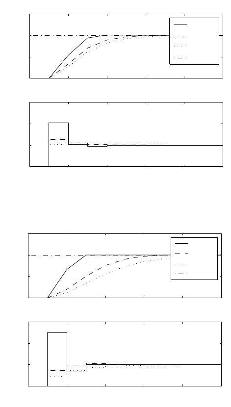
Two simulation runs were performed. In the ﬁrst, mean level settings were

given. The GPC parameters were N

=1,N

=1,λ =0,andN

varied

between 2 − 20. The results are shown in Fig. 9.4 and illustrate that with

the increasing N

the control actions are smoother, more conservative and

converge to input step change.

In the second simulation λ was given as the varying parameter. The set-

tings of other parameters were N

=3,N

= 5 which for λ = 0 gives

the dead-beat controller. Increasing λ gives more weight to control increments

and slows down the controller. The results are shown in Fig. 9.5.

9.8 Examples 437

0 2 4 6 8 10

0.5

1.5

Output

y,w

=20

0 2 4 6 8 10

Control

sam

Fig. 9.4. Increasing value of N

leads towards mean-level control

0 2 4 6 8 10

0.5

1.5

Output

y,w

λ=0.0

λ=0.1

λ=1.0

0 2 4 6 8 10

Control

sample

Fig. 9.5. Increasing value of λ - detuned dead-beat control

438 9 Predictive Control

9.8.2 Neural Network based GPC

In this example we compare an adaptive GPC based on linear model (AGPC)

and implemented in the same way as in the previous example to GPC based

on non-linear neural network model (GPCNN).

The process studied was the bioprocess that describes the growth of Sac-

charomyces cerevisiae on glucose. The oxygen concentration c

and the dilu-

tion rate D

have been selected as the controlled and the manipulated vari-

ables, respectively.

A feedforward ANN plant model with the third order input dynamics and

one hidden layer was used. This means six neurons in the input layer with

signals

y(k − 1),y(k − 2),y(k − 3),u(k − 1),u(k − 2),u(k − 3) (9.151)

For the calculation of the step response, the ANN inputs are

y(k − 1),y(k − 1),y(k − 1),u

,u(k − 1),u(k −1) (9.152)

where the step change magnitude u

was speciﬁed as

= u(k − 1) +

w − y(k − 1)

(9.153)

and the process static gain Z was determined from the step response estimated

in the previous sampling period. The static gain Z was initially set equal to

1. To take into account the fact that the initial conditions are not equal to

zero and the step input is not of unit value, the ANN approximation of the

step response is subsequently normalised.

For the free response the ANN inputs are

u(k − 1),u(k − 2),u(k − 3),y(k − 1),y(k − 2),y(k −3) (9.154)

and it is assumed that the input is constant in the future.

The sampling period was set equal to 0.5 h. The training and validation

data sets (800 input-output pair samples) were obtained using a pseudo ran-

dom binary sequence input. The conjugate gradients algorithm was used as a

learning method and a genetic algorithm was used for the initialization of the

ANN weights.

For the AGPC, a third order discrete model has been considered for process

modelling. The model parameters have been estimated using the parameters

estimation algorithm LDDIF.

The GPC parameters were N

=1,N

=14,N

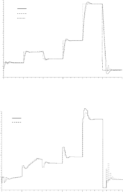
=4,λ =0.1. The ob-

tained proﬁles of the process output controlled by the AGPC (dashed line)

and the GPCNN (solid line) are shown in Fig. 9.6. Figure 9.7 shows the pro-

ﬁles of the control actions generated by AGPC (dashed line) and GPCNN

(solid line), respectively. As it can be seen from these ﬁgures, both algorithms

9.8 Examples 439

0 102030405060

0,0

0,3

0,6

0,9

1,2

1,5

1,8

2,1

- GPCNN

- AGPC

. 10

[ mol / l ]

Time [ h ]

Fig. 9.6. Trajectories of the oxygen concentration (the process output)

0 102030405060

0,0

0,2

0,4

0,6

0,8

1,0

1,2

1,4

Dg - GPCNN

Dg - AGPC

Control action Dg [1/h]

Time [ h ]

Fig. 9.7. Trajectories of the dilution rate (the manipulated variable)

achieve good results. When a large change of the setpoint occurs (see Fig. 9.7,

t = 50 h), GPC based on linear model leads to a generation of a bad transient

behaviour. Unlike AGPC, GPC based on ANN generates a smooth control

action which leads to a good control behaviour. This behaviour was expected

as the AGPC is based on linear model. Due to the nonlinear characteristic of

the bioprocess, a large change of the setpoint or some disturbance can bring

the process into other operating points with diﬀerent dynamical properties.

9.8.3 pH Control

The experimental pH control has been studied at the University of Dortmund.

440 9 Predictive Control

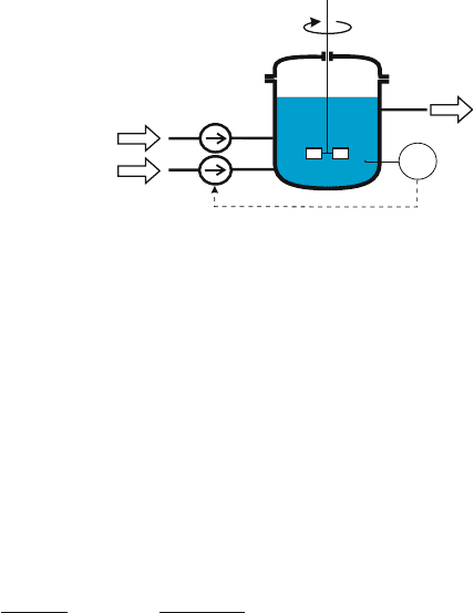
The neutralisation plant to be controlled consists of a laboratory-scale

continuous stirred tank with two inlets and one outlet (see Fig. 9.8)), in which

acetic acid is neutralized with sodium hydroxide.

The hold-up of the tank is 5.57 l, the concentrations of the acid and the

sodium hydroxide solution streams are approximately 0.01 mol/l. The acid

ﬂow rate F

is ﬁxed at 0.33 l min

−1

, whereas the NaOH ﬂow F

is manipulated

by the controller. In order to obtain the necessary precision of the ﬂow rates

diaphragm pumps were chosen. All control actions are performed by a PC-

based control system. The ﬂow F

is controlled by the modulation of an

impulse frequency f, which leads to a quantisation of the control amplitude

because the frequency can assume only certain discrete values.

acetic acid

sodium

hydroxide

efluent

stream

QIC

Fig. 9.8. Neutralisation plant

In the tank, the following reaction takes place:

NaOH + CH

COOH  CH

COONa + H

O (9.155)

Due to the incomplete dissociation of the acetic acid in water and the

equilibrium reaction with sodium hydroxide the system behaves like a buﬀer

solution between pH 4 and 6.5. Consequently, the process gain varies extremely

over the range of pH-values that can be controlled.

The controlled variable pH and the control variable F

have been scaled

for control and identiﬁcation purposes as

y =

pH −7

u =

− F

(9.156)

where F

denotes the approximate steady state value of F

corresponding to

pH = 7.

The parameters for the GPC controller were chosen as N =50,N

4,λ =1,α =0.3. Several model orders have been tried, the best results have

been obtained with the third order model. The sampling time was set at 5s.

The tuning of the predictive algorithm was performed at pH = 9 with

the requirement, that the deviations from the steady-state have to be within

9.8 Examples 441

±0.1pH. It was observed, that the small values of N

led to rather active con-

trol actions and the ﬁnal value N

= 4 was chosen as the result of trade-oﬀ

between the performance and the complexity of the calculations. The param-

eter λ inﬂuenced the penalisation of the future control increments. Very large

values caused limit cycles of pH as the control was unable to compensate sat-

isfactorily the disturbances, therefore the smallest possible value was chosen.

For the ﬁnal tuning of the algorithm, the P polynomial was used. Only

the ﬁrst order polynomial of the form P (z

−1

)=(1− αz

−1

)/(1 − α)was

assumed. The smaller values resulted in increased steady-state deviations and

the larger values in very slow and oscillatory response to setpoint changes.

The value α =0.3 was chosen as a compromise.

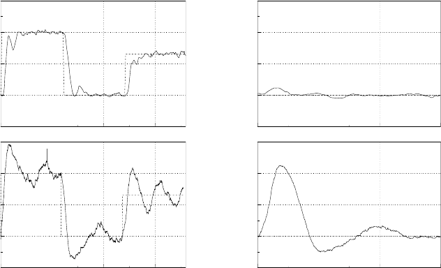
The experimental results of the adaptive GPC controller were compared

with a carefully tuned PI controller. All experiments were carried out with the

same pattern of setpoint changes. At ﬁrst the reactor was stabilised at pH = 7

and then controlled to pH = 9, 7, 8.3 (Fig. 9.9). Finally, the disturbance

rejection performance has been studied. As a disturbance, a 20% decrease

of the acid ﬂow was performed at t = 0 and held constant afterwards (see

Fig. 9.10).

0 500 1000 1500

PI controller

pH [ ]

Time [s]

GPC controller

pH [ ]

Fig. 9.9. Setpoint tracking

0 200 400 600

PI controller

pH [ ]

Time [s]

GPC controller

pH [ ]

Fig. 9.10. Disturbance rejection

The experiments have conﬁrmed, that the adaptive GPC method is able to

control the strongly nonlinear plant and that it behaves much better compared

to the linear PI control. However the tuning of the controller parameters

must have been done with some care and only the parameters which slowed