Mikles J., Fikar M. Process Modelling, Identification, and Control

Подождите немного. Документ загружается.

412 9 Predictive Control

AΔ + P

−1

CAΔ + z

−1

AΔ

j=N

+ Bz

−1

j=N

(9.50)

CAΔ + z

−1

j=N

(AΔΓ

+ BF

)

j=N

(9.51)

= C

AΔ +

j=N

j−1

(B − AΔG

)

j=N

(9.52)

= CM (9.53)

We can see that the characteristic polynomial is composed of two polynomials.

The ﬁrst determines the behaviour of the closed-loop system with respect to

disturbances and corresponds to the observer poles. The second polynomial

depends in a rather complicated way on the controlled process and the GPC

parameters. It determines the closed-loop stability as it can also be seen from

the output equation

y(z)=

−1

w(z)+

ξ(z) (9.54)

where the polynomial C has been cancelled in both transfer functions.

9.3.4 Derivation of the Predictor from State-Space Models

To show that it is possible to use any linear model, we will derive here the

predictor equations based in the state-space model.

Let us consider the standard state-space model of the form (9.4), (9.5).

Like in the previous case when CARIMA model was used, it is necessary to

include an integrator to the process. This can be accomplished by changing

the input to the process from u(k) to its increment Δu(k)

u(k)=Δu(k)+u(k − 1) (9.55)

There are more possibilities how to incorporate an integrator in the process

model. Among them, one way is to deﬁne a new state vector

¯x(k)=



x(k)

u(k − 1)



(9.56)

From the state-space model (9.4), (9.5) then follows

¯x(t +1)=



0 I



¯x(k)+





Δu(k)=

A¯x(k)+

BΔu(k) (9.57)

y(k)=



C 0



¯x(k)=

C ¯x(k) (9.58)

We can see that formally both state-space models are equivalent.

9.3 Derivation and Implementation of Predictive Control 413

The derivation of the predictor is simpler than in the input-output case.

The predictor vector is given as

y(t +1)=

C ¯x(t +1)=



A¯x(k)+

BΔu(k)



(9.59)

y(t +2)=

C ¯x(t +2)=



A¯x(t +1)+

BΔu(t +1)



(9.60)

y(t + N

C ¯x(t + N



A¯x(t + N

− 1) +

BΔu(t + N

− 1)



(9.61)

where the state predictions are of the form

¯x(t +1)=

A¯x(k)+

BΔu(k) (9.62)

¯x(t +2)=

A¯x(t +1)+

BΔu(t +1)

¯x(k)+

BΔu(k)+

BΔu(t + 1) (9.63)

¯x(t + N

¯x(k)+

−1

BΔu(k)+···+

BΔu(t + N

− 1) (9.64)

Joining all predictions to form the vector equation (9.34) yields matrices and

vectors

G =

⎛

⎜

⎝

B 0 ... ... 0

B 0 ... 0

B 0

−1

B ... ...

⎞

⎟

⎠

(9.65)

and

⎛

⎜

⎝

⎞

⎟

⎠

¯x(k) (9.66)

Example 9.1:

To explain the principle let us consider a simple SISO process with the

numerator and denominator polynomials of the form

B(z

−1

)=0.4+0.1z

−1

,A(z

−1

)=1− 0.5z

−1

This corresponds to the process transfer functions of the form

0.4z

−1

+0.1z

−2

1 −0.5z

−1

Let us assume that C(z

−1

) = 1. The CARIMA description of the system

is of the form

414 9 Predictive Control

ΔA(q

−1

)y(k)=B(q

−1

)Δu(k − 1) + ξ(k)

y(k)=1.5y(k −1) −0.5y(k −2) + 0.4Δu(k −1) + 0.1Δu(k −2) + ξ(k)

Let us now assume the cost function (9.8) with the parameters N

=1,

=3,N

=2.

The predictions of future outputs can be obtained if ξ(t + i) = 0 and are

as follows:

ˆy(t +1)=1.5y(k) −0.5y(k − 1) + 0.4Δu(k)+0.1Δu(k − 1)

ˆy(t +2)=1.5y(t +1)− 0.5y(k)+0.4Δu(t +1)+0.1Δu(k)

ˆy(t +3)=1.5y(t +2)− 0.5y(t +1)+0.4Δu(t +2)+0.1Δu

(t +1)

According to the assumptions, the term Δu(t + 2) is equal to zero. The

higher output predictions contain the lower output predictions that can

be back substituted and yield

ˆy(t +1)=1.5y(k) −0.5y(k − 1) + 0.4Δu(k)+0.1Δu(k − 1)

ˆy(t +2)=1.75y(k) −0.75y(k − 1)

+0.4Δu(t +1)+0.7Δu(k)+0.15Δu(k − 1)

ˆy(t +3)=1.875y(k) −0.875y(k

− 1)

+0.7Δu(t +1)+0.85Δu(k)+0.175Δu(k − 1)

Stacking all predictions into a vector and separating the terms unknown

at time k from the known ones gives

⎛

⎝

ˆy(t +1)

ˆy(t +2)

ˆy(t +3)

⎞

⎠

⎛

⎝

0.40

0.70.4

0.85 0.7

⎞

⎠



Δu(k)

Δu(t +1)



⎛

⎝

1.5y(k) − 0.5y(k − 1) + 0.1Δu(k − 1)

1.75y(k) − 0.75y(k − 1) + 0.15Δu(k − 1)

1.875y(k) − 0.875y(k − 1) + 0.175Δu(k − 1)

⎞

⎠

An alternative to obtain the matrix G would be to perform the long

division

ΔA

0.4+0.1z

−1

1 −1.5z

−1

+0.5z

−2

=0.4+0.7z

−1

+0.85z

−2

+ ···

Now let us assume that the weighting coeﬃcient λ is equal to zero. Inver-

sion of the Hessian matrix gives

−1



5.1383 −6.9170

−6.9170 10.8498



Finally, multiplication with g yields the closed-loop expression for the

element

Δu(k)=−3.6461y(k)+1.2351y(k − 1) −0.2470Δu(k − 1)

+2.0553w(t +1)+0.8300w(t +2)− 0.4743w(t +3)

9.3 Derivation and Implementation of Predictive Control 415

0 2 4 6 8 10

0.5

1.5

Output

y,w

0 2 4 6 8 10

Control

sam

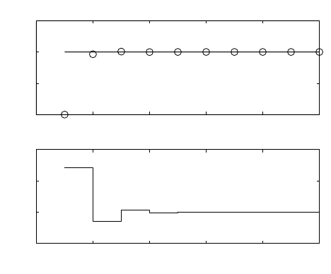
Fig. 9.2. Closed-loop response of the controlled system

Simulation results show the behaviour of the closed-loop system in the

Fig. 9.2.

Let us also derive the predictor equations in the state-space form. The

corresponding state-space model can for example be given as

x(t +1)=



00.5



x(k)+





u(k)

y(k)=



0.10.4



x(k)

The new state-space description with integrator has three states

¯x(t +1)=

⎛

⎝

010

00.51

001

⎞

⎠

¯x(k)+

⎛

⎝

⎞

⎠

Δu(k)=

A¯x(k)+

BΔu(k)

y(k)=



0.10.40



¯x(k

C ¯x(k)

The state predictions of three steps to the future are then given as

¯x(t +1)=

A¯x(k)+

BΔu(k)

¯x(t +2)=

A¯x(t +1)+

BΔu(t +1)

¯x(k)+

BΔu(k)+

BΔu(t +1)

¯x(t +3)=

A¯x(t +2)

¯x(k)+

BΔu(k)+

BΔu(t +1)

The output predictions are then given as

ˆy(t +1)=

A¯x(k)+

BΔu(k)

ˆy(t +2)=

¯x(k)+

BΔu(k)+

BΔu(t +1)

ˆy(t +3)=

¯x(k)+

BΔu(k)+

BΔu(t +1)

or in the vector form

416 9 Predictive Control

⎛

⎝

ˆy(t +1)

ˆy(t +2)

ˆy(t +3)

⎞

⎠

⎛

⎝

B 0

⎞

⎠



Δu(k)

Δu(t +1)



⎛

⎝

⎞

⎠

¯x(k)

When the actual values are substituted for the system matrices and states,

it yields

⎛

⎝

ˆy(t +1)

ˆy(t +2)

ˆy(t +3)

⎞

⎠

⎛

⎝

0.40

0.70.4

0.85 0.7

⎞

⎠



Δu(k)

Δu(t +1)



⎛

⎝

0.3x

(k)+0.4u(k − 1)

0.15x

(k)+0.7u(k − 1)

0.075x

(k)+0.85u(k − 1)

⎞

⎠

We can note that the matrix G is the same in both cases. The second part

depends on the actual state deﬁnitions. However, the predictive controller

will be the same.

9.3.5 Multivariable Input-Output Case

In the same line of thought as in the SISO case, the multivariable GPC algo-

rithm can de derived via Diophantine equations. From the practical point of

view, the multivariable controller can come from the prediction equation (9.22)

that holds exactly as before, only the vector and matrix elements instead of

being scalar are vectors and matrices. If m-input and n-output system is con-

sidered, then the matrix G is of the form

G =

⎛

⎜

⎝

0 ... ... 0

0 ... 0

. G

−1

... ... G

⎞

⎟

⎠

(9.67)

with G

being matrices of dimensions [n×m] and the overall G has dimensions

[n(N

− N

+1)× mN

The vectors y

and matrices G

can be obtained analogously as in the

singlevariable case from free and step responses of the system.

The drawbacks of the proposed multivariable derivation are increased di-

mensions of the matrices involved in matrix inversion routines. The multivari-

able formulation can be broken into series of SISO GPC calculations if the

system denominator matrix A(z

−1

) is diagonal.

9.3.6 Implementation

As it was stated before, for the actual implementation of the linear GPC

algorithm only two process characteristics are needed: step and free responses.

The step response can be obtained directly from the process by performing a

9.3 Derivation and Implementation of Predictive Control 417

small step change in one of the manipulated inputs at a time if the process

was before in a steady state. The magnitude of the step change is important

if the process is non-linear. If the process steady-state gain is approximately

known then the magnitude of the input step change should be chosen such

that it produces step response approaching the desired setpoint value. This

strategy may be applied if a non-linear model is used for predictions.

If the polynomials A, B are estimated on-line by means of a RLS algorithm,

the step response is obtained from the polynomial division

AΔ

= g

+ g

−1

+ ···+ g

−N

+ ···+ g

−N

+ ··· (9.68)

The matrix G can be formed from the coeﬃcients of the step response and it

is given by the last N

−N

+ 1 rows and the ﬁrst N

columns of the Toeplitz

matrix (9.33).

The free response is calculated as the process response from the actual

initial conditions if the input is ﬁxed to u(k − 1). At time k is should hold

y(k)=y

(k) (9.69)

However, the assumption about random-walk disturbance usually results in

non-zero disturbance at time k and holds

y(k)=y

(k)+d(k) (9.70)

This disturbance is assumed to be constant in all future predictions. The

disturbance and the free response are thus calculated as

d =

deg(A)



i=0

(k − i) −

deg(B)



i=0

(k − i − 1) (9.71)

(t + j)=y

(t + j) (9.72)

= d −

deg(A)



i=1

(k − i + j)+

deg(B)



i=0

¯u(k − i + j − 1) (9.73)

where

¯u(k − i + j)=



(k − 1) j ≥ i

(k − i + j) inak

(9.74)

and

(9.75)

Note 9.1. If polynomial P is assumed to be non-unity, then the above is valid

if the system denominator A is changed for PA. To ensure the oﬀset-free

setpoint following, the polynomial P should be speciﬁed subject to condition

P (1) = 1.

418 9 Predictive Control

Note 9.2. The polynomial C is normally not estimated on-line, but used as a

user-design parameter. It can be shown from relation between state-space and

input-oputput approaches that it acts as an observer polynomial and is used

for disturbance rejection.

9.3.7 Relation to Other Approaches

One of the features of GPC approach is its generality. With diﬀerent values

of its parameters it can be reduced to some well-known controllers:

Mean level control

=1,N

→∞,N

=1,P=1,λ=0

Exact model following

=1,N

= T

+1,N

= T

+1,P=1,λ=0

=1,N

= N

− T

,P=1,λ=0

Dead-beat control

≥ deg(B)+1,N

≥ N

+ N

−1,N

≥ deg(A)+1,P=1,λ=0

Pole placement Dead-beat + P . Poles are placed at zeros of P .

≥ deg(B)+1,N

≥ N

+ N

−1,N

≥ deg(A)+1,P=1,λ=0

9.3.8 Continuous-Time Approaches

Predictive control has been developed in discrete-time domain. The discrete

formulation allows for an easy prediction generation, because time response

of discrete systems can be obtained from polynomial division of the system

numerator and denominator.

The analogical formulation for continuous-time systems is by no means so

simple. The principial polynomial equations remain the same, however, their

interpretation is diﬀerent. For the signal predictions, the Taylor expansion is

used. However, the main advantage of MBPC – constraints handling, is very

diﬃcult with this approach.

There are some approaches that are more realistic while still allowing con-

straints. The main principle is to approximate the future control and output

signals as a linear combination of selected continuous-time base functions –

for example splines. The real optimised variables become parameters of the

splines. It can be shown that both input and output signal approximations

9.4 Constrained Control 419

are aﬃne functions of these parameters and thus constrained continuous-time

predictive control can be solved as a Quadratic Programming task.

The advantage of this approach is a truly continuous-control where the

choice of the sampling time is not so crucial as in the discrete time case. For

the disadvantages, we mention a larger number of user parameters and not

very clear stability properties.

9.4 Constrained Control

The GPC algorithm derived in the preceding section did not consider the

presence of constraints. This is not very realistic, as in practice some kind of

constraints is usually present in the process control. Most often, inputs are

constrained to be between some minimal and maximal values (ﬂows cannot

be negative, valves can be opened at 100% maximally) or input rate changes

are limited. Usually, there also exist some recommended values of process

outputs; these are often formulated as soft constraints as opposed to hard

input constraints.

The ability to handle constraints is one of the key properties of MBPC and

also caused its spread, use, and popularity in industry. Nowadays, most of the

industrial processes run at the constraints, if not, the process is unnecessarily

overdesigned.

One might argue that input constraints can be respected if the calculated

control by some control method is subsequently clipped to be within limits.

There are at least two reasons not to do so:

• There is a loss of anticipating action. As the control is on its limit, it

cannot inﬂuence the process in a suitable way (one degree of freedom is

lost). The process may go totally unstable, out of limits of safety, or to

an emergency mode. This usually causes heavy economic losses connected

with emergency stop and start-up procedures.

• If multivariable control is considered, certain inﬂuence between the input

vector elements has to be respected. Clipping one input element may cause

entirely diﬀerent transient responses. This phenomenon is called direction-

ality of a multivariable plant.

The cost function used in GPC is quadratic and of the form (9.35). If we

assume only constraints that are linear with respect to the optimised vec-

tor ˜u then the resulting optimisation problem may be cast as the Quadratic

Programming problem which is known to be convex and for which eﬃcient

programming codes exist. The general constrained GPC formulation is thus

given as

min

˜u

˜u + ˜u

H ˜u subject to: A˜u ≥ b (9.76)

Several types of constraints may be written in this general form:

420 9 Predictive Control

Input rate limits Δu

min

≤ Δu ≤ Δu

max

A =



−I



, b =



1Δu

min

−1Δu

max



where 1 is a vector whose entries are ones.

Input amplitude limits u

min

≤ u ≤ u

max

A =



−L



, b =



min

− 1u(t − 1)

−1u

max

+ 1u(t − 1)



where L is a lower triagonal matrix whose entries are ones.

Output constraints y

min

≤ y ≤ y

max

A =



−G



, b =



min

− y

−y

max

+ y



Several other types of output constraints can be handled similarly: overshoot,

undershoot, monotony, etc.

Although input constraints can always be met, presence of output con-

straints can cause infeasibility of the Quadratic Programming. Therefore from

practical point of view, hard output constraints should be changed to soft con-

straints where amount ε of constraint violation is penalised. In such a case

the output constraints are of the form

−ε + y

min

≤ y ≤ y

max

− ε, ε > 0 (9.77)

and the cost function (9.35) is of the form

I =2g

˜u + ˜u

H ˜u + ε

Hε (9.78)

and the variables ε are added to optimised variables.

9.5 Stability Results

Any predictive method minimising the ﬁnite horizon cost function may become

unstable in some cases. This can easily be imagined if the system controlled

contains right half plane zeros, the output horizon is equal to one, and control

penalisation is equal to zero. Inevitably, the predictive controller that min-

imises only the output error, is able to set it to zero at each sampling time.

The price however is, that the control signals are increasing in magnitude and

the system will be unstable.

This is one of the main issues against MBPC. Although the methods may

work well in practice, some systems exists in theory for which the methods

are highly sensitive. Even more signiﬁcant is, that there is no clear theory

which predicts the closed-loop behaviour for arbitrary horizons and control

penalisations.

9.5 Stability Results 421

Therefore, two main streams toward stability have been developed. In the

ﬁrst case, some combinations of GPC parameters have been proven to be

stabilising. The second line of research has been devoted to methods that

overcome the basic GPC drawbacks.

9.5.1 Stability Results in GPC

Theorem 9.3. The closed-loop system is stable if the system is stabilisable

and detectable and if:

• N

→∞, N

= N

,andλ>0 or

• N

→∞, N

≤ N

− n +1,andλ =0where n is the system

state dimension.

Theorem 9.4. For open-loop stable processes the closed-loop system is stable

and the control tends to a mean level law for N

=1and λ =0as N

→∞.

Theorem 9.5. The closed-loop system is equivalent to a stable state dead-beat

controller if

1. the system is observable and controllable and

2. N

= n, N

≥ 2n − 1, N

= n,andλ =0where n is the system state

dimension.

9.5.2 Terminal Constraints

The ﬁrst approach that forces MBPC methods to be stable is based on the

state terminal constraints. Roughly speaking, the system is stable if it is sub-

ject to the moving-terminal constraint on ﬁnal states

x(k + N

)=0 (9.79)

Several diﬀerent algorithm have emerged that are based on this result.

CRHPC

CRHPC (Constrained Receding Horizon Predictive Control), and SIORHC

(Stable Input Output Receding Horizon Control) were developed indepen-

dently, but are in fact equivalent. The idea behind these techniques is an

equivalent of the state terminal constraint within input/output system de-

scription. Hence, these methods optimise the usual quadratic function over

ﬁnite horizons subject to condition that the output exactly matches a ref-

erence value over a future constraint range (after k + N

). Some degrees of

freedom force the output to stay at setpoints while the remaining degrees of

freedom are available to minimise the cost function. The output constraint

description is